Magnetic Anomaly Maps
IEEE/ION PLANS 2023, Monterey, CA
The views expressed in this article are those of the author and do not necessarily reflect the official policy or position of the United States Government, Department of Defense, United States Air Force or Air University.
Distribution A: Authorized for public release. Distribution is unlimited. Case No. 2023-0277.
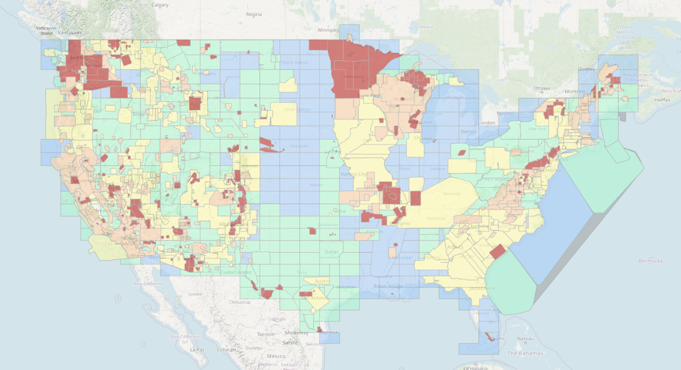
Airborne magnetic anomaly surveys
- Usually performed in smaller area for geological interpretation
- Large anomaly maps merged together in mosaic using a leveling process
- Meant to merge long spatial wavelengths
- Many anomaly surveys pre-date GPS
- Geolocated via air-crew observations
- Typically remove space-weather effects with ground-station
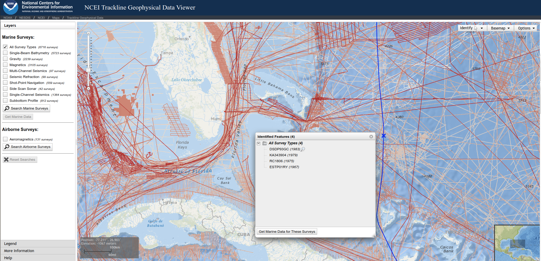
Marine track surveys
- Often single long track following ship
- Many pre-date GPS
- Use ship’s positioning
- Typically no space weather correction
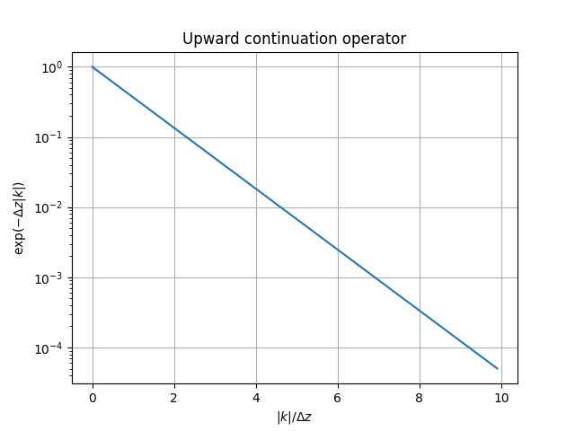
Upward continuation
Magnetic anomaly maps are usually made at a single altitude.
The process of taking a magnetic map from one altitude to another.
- \(F(B_\text{up}) = F(B_\text{known}) e^{-\Delta z |k|}\)
- Assumes a flat Earth model with all the sources below
- (Blakely 1995)
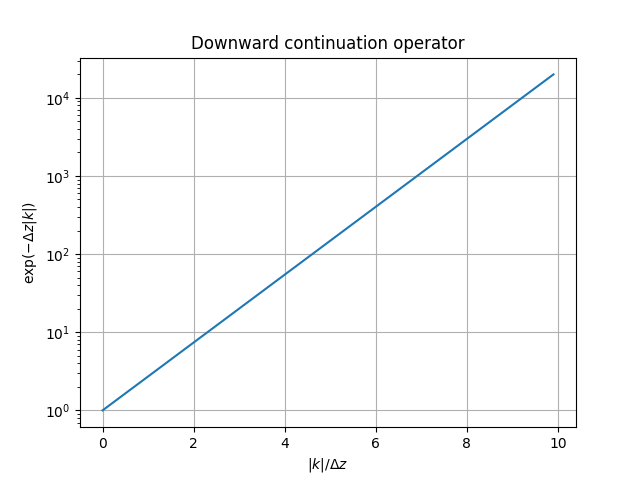
Dangerous downward continuation
The process of taking a magnetic map from one altitude to another.
- \(F(B_\text{down}) = F(B_\text{known}) e^{+\Delta z |k|}\)
- Noise can be amplified
- Techniques to do this exist, and involve some kind of regularization or source estimation
- (Blakely 1995)
Scalar Potential Theory
A procedure to transform magnetic scalar potential \(\Phi_M\) in free space.
From Laplacian we can write (Green’s third identity) \[
\Phi_M(\vec{r}) = \frac{1}{4\pi} \int_S \left( \frac{1}{r} \frac{\partial \Phi_M}{\partial n} -
\Phi_M \frac{\partial}{\partial n} \frac{1}{r} \right) dS
\]
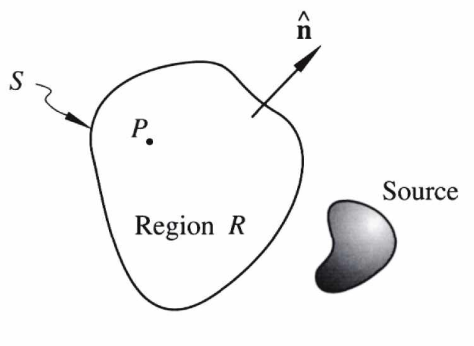
- No sources in region \(R\)
- Know \(\Phi_M\) on the surface \(S\) that bounds \(R\)
- We can find \(\Phi_M\) anywhere in \(R\)
- (Blakely 1995)
Hemispherical geometry - flat Earth model
- Think of Earth’s surface as an infinite flat plane, all sources below
- Measure the potential on a plane above the earth
- Other side of hemisphere is \(\infty\) away and therefore zero potential
- Potential anywhere inside can be computed
Fourier methods for potential theory
- Goal: find the potential \(\Phi_M\) on a plane parallel to a known plane
- Process: double integral over the surface of the known plane
- Ends up looking like a 2-D Fourier transform over spatial coordinates
- (Blakely 1995)