drms (generic function with 1 method)Magnetic Anomaly Navigation Tutorial
IEEE/ION PLANS 2023, Monterey, CA
The views expressed in this article are those of the author and do not necessarily reflect the official policy or position of the United States Government, Department of Defense, United States Air Force or Air University.
Distribution A: Authorized for public release. Distribution is unlimited. Case No. 2023-0277.
Schedule
Tutorial is 90 minutes total:
- 40 minutes
- 10 minutes break
- 40 minutes
Outline
Magnetic Anomaly Navigation Overview
Requirements for MagNav
Discuss publicly available MagNav software and dataset
Learn and perform traditional aircraft calibration
- Tolles-Lawson
Evaluate navigation performance
Calibration/noise removal
Navigation performance improvement
Magnetic Anomaly Navigation Overview
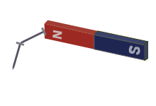
Refrigerator magnet 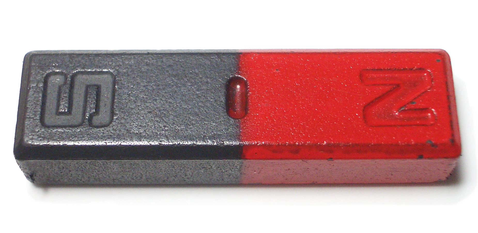
Earth’s core field (compass) 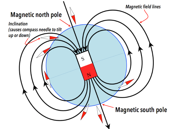
Crustal magnetic anomaly 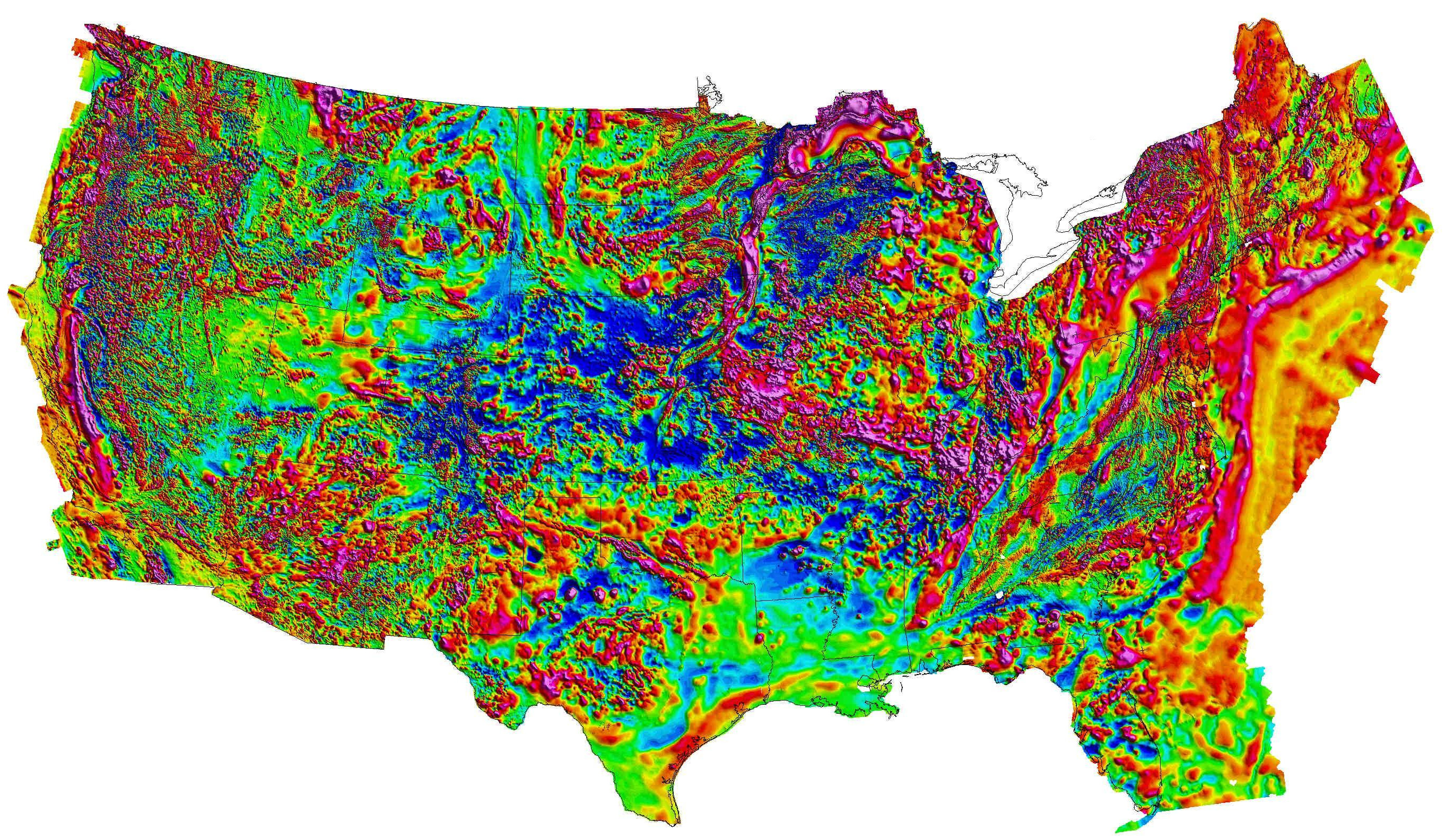
1 000 000 nT
Range \(\pm\) 500 nT
Resolution \(\sim\) 1 nT https://mrdata.usgs.gov/magnetic/ (Bankey et al. 2002)
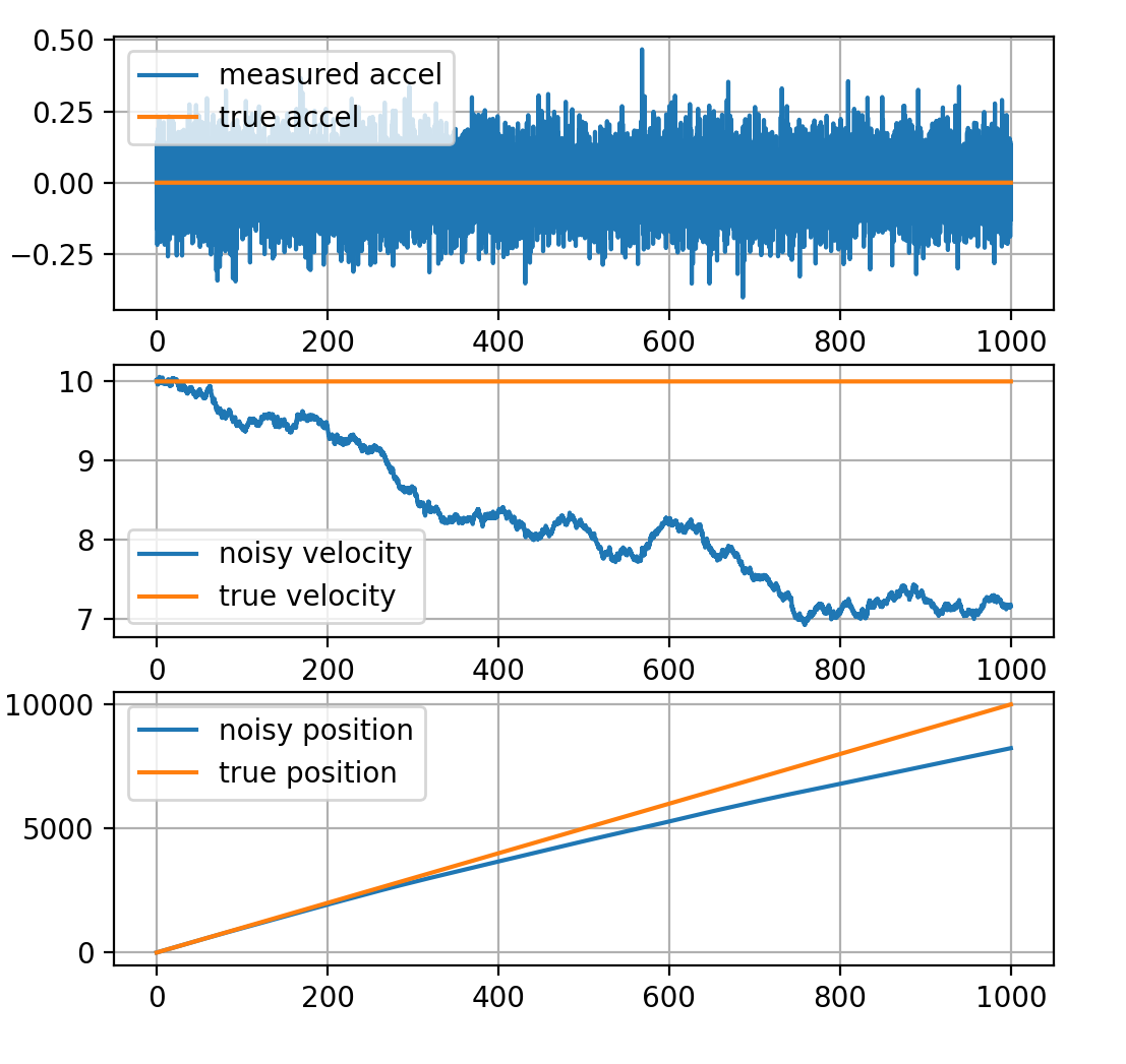
Inertial Navigation
Inertial Measurement Unit (IMU)
- measures accelerations
- measures rotation rates
To get position from accleration, you have to integrate twice
- continuously adds noise to your position estimate
Drifting position estimate needs to be corrected
- Magnetic Anomaly Navigation matches to magnetic anomaly map
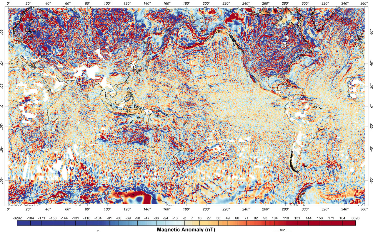
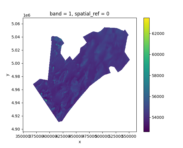
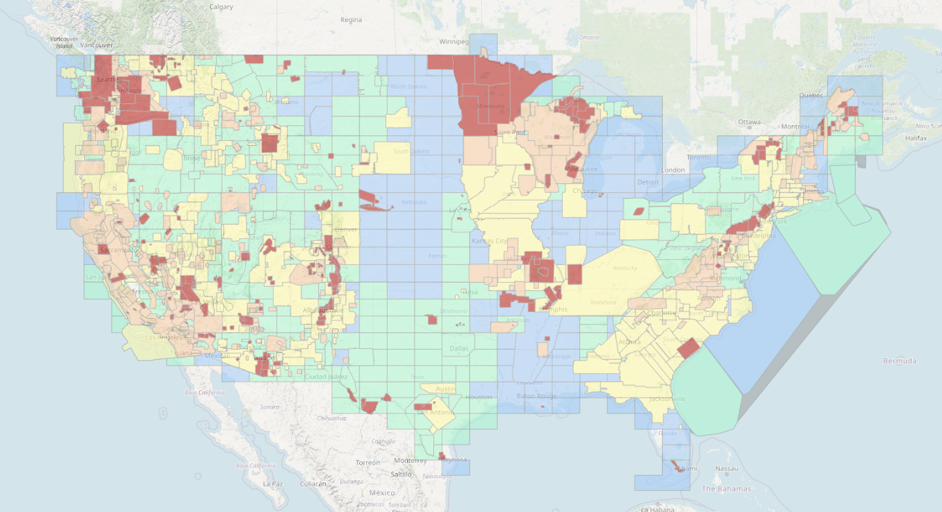
Earth Magnetic Anomaly Grid 2-arcsec v3
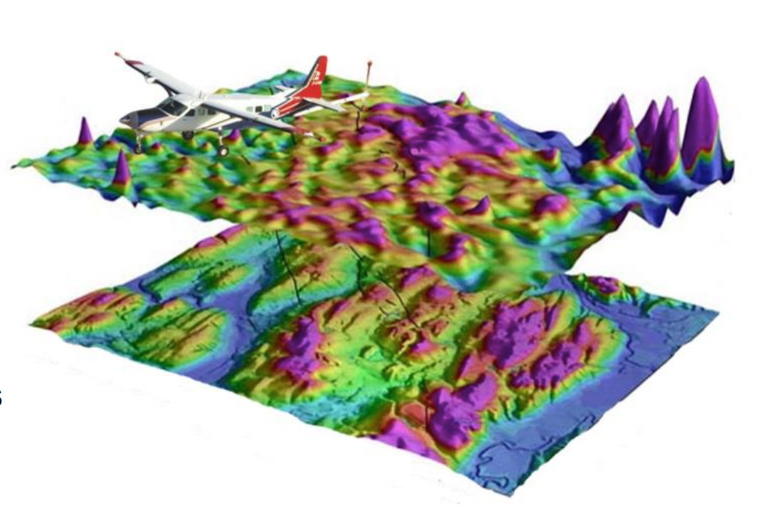
Map-based navigation
Features are required to navigate
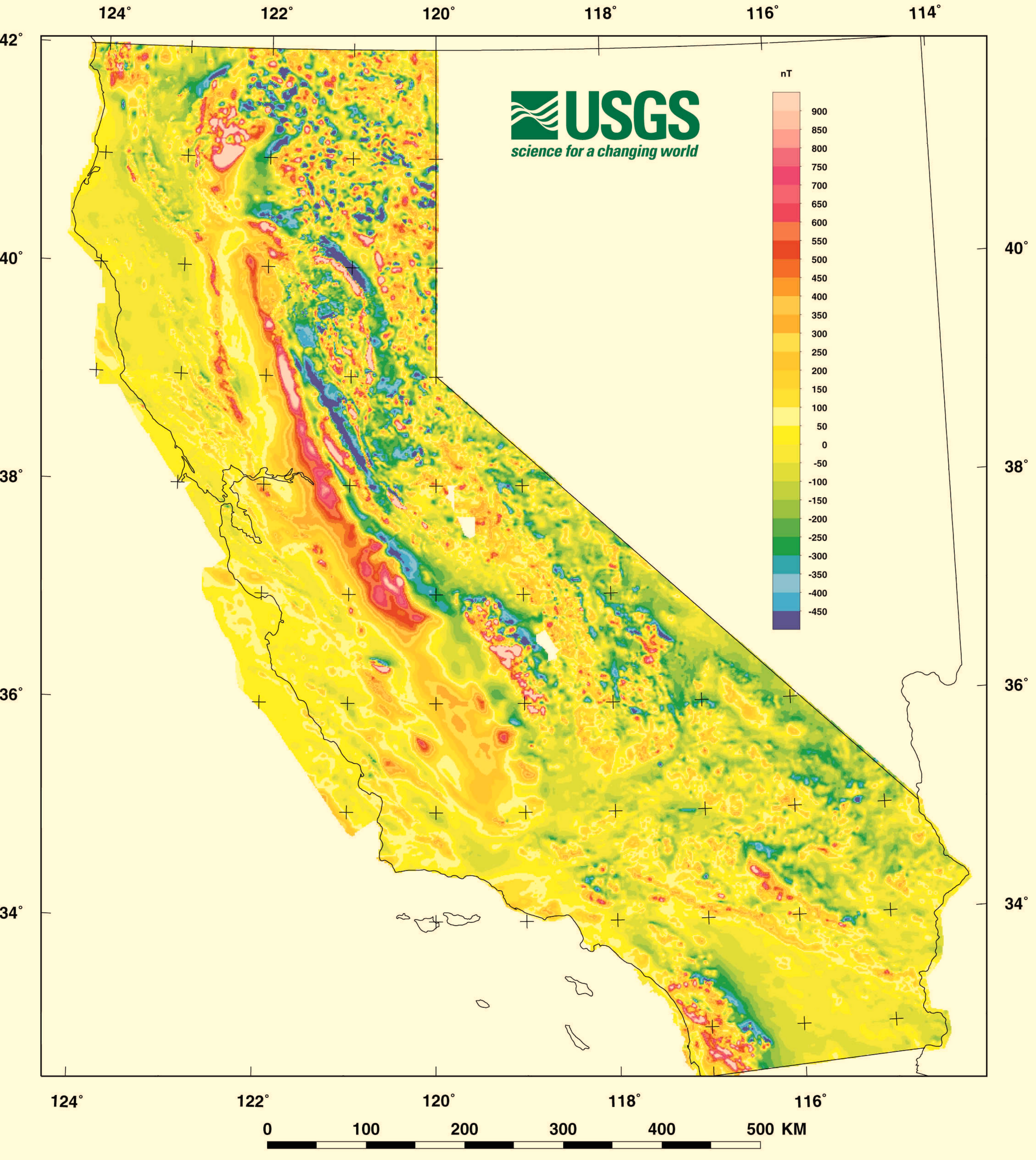
Magnetic anomaly closely tied to geology
- less variation in coastal region
- direction variation in Central Valley
- more structure in Sierra Nevada mountains
Area and direction of travel make a difference
Interpretation of magnetic anomaly
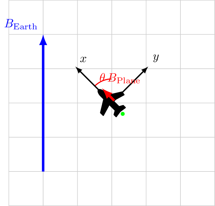
-The primary sensor used is a scalar magnetometer which measures: \(|\vec{B}|\)
-The field is a vector \(\vec{B}\)
-Interpretation of \(|\vec{B}|\) relies on understanding
\(|\vec{B}_\sensor| = |\vec{B}_\earth + \vec{B}_\text{anomaly}|\)
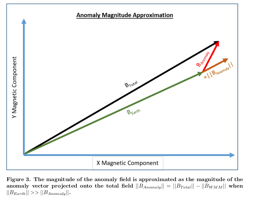
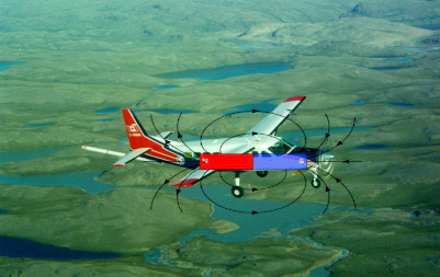
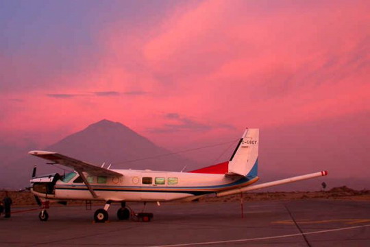
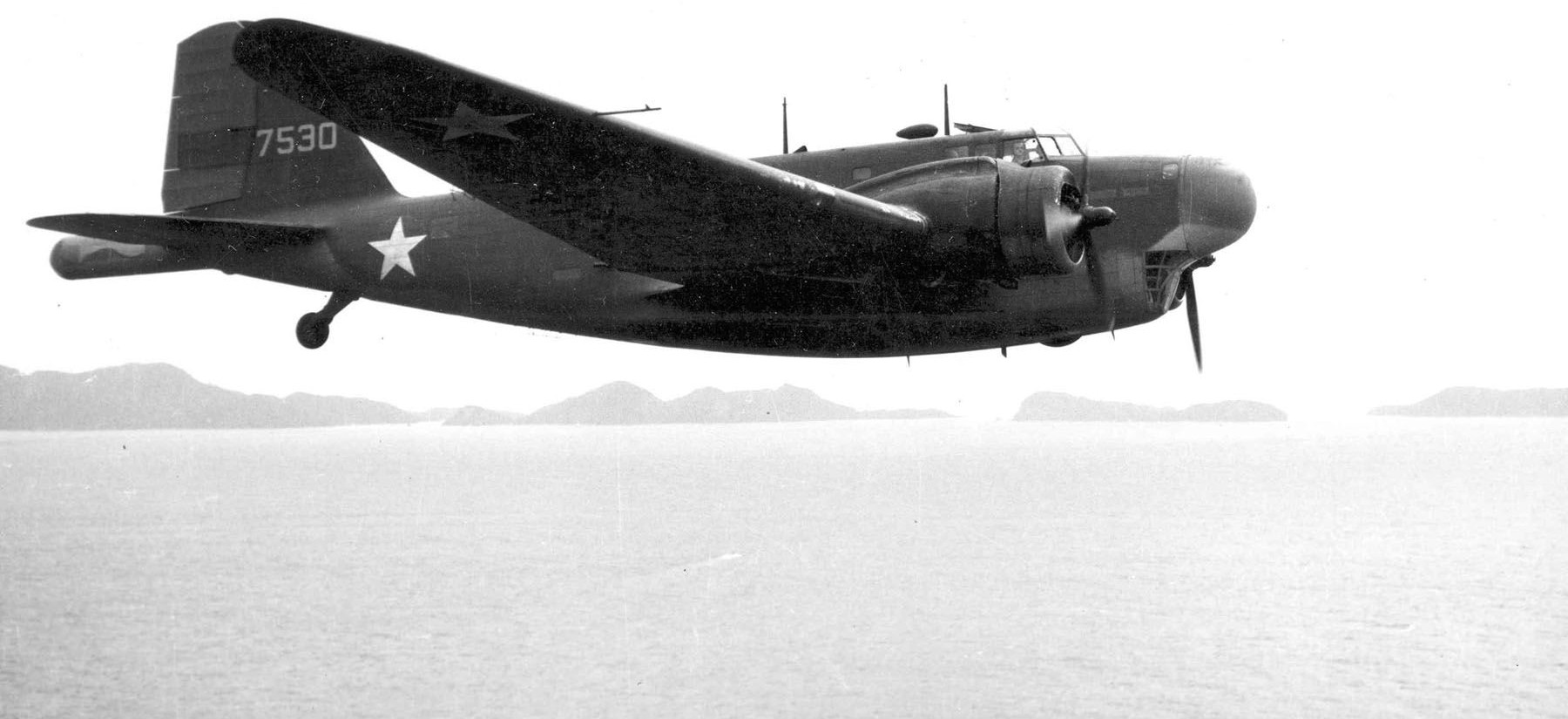
An airplane is a big magnet that flies
\(|\vec{B}| = |\vec{B}_\earth + \vec{B}_\text{anomaly} + \vec{B}_\plane|\)
Aircraft Calibration
Sensor placement and installation
- Engineered location
- Stinger
- Survey for placement
- Non-magnetic fasteners
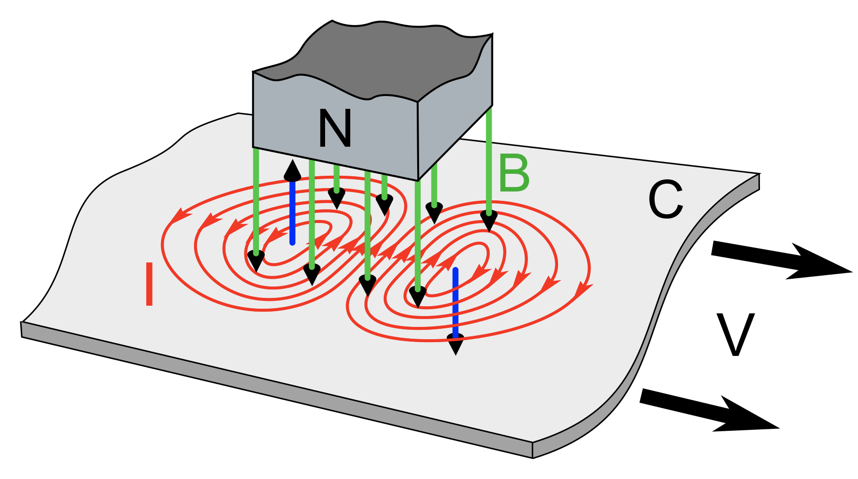
Degaussing
Algorithms

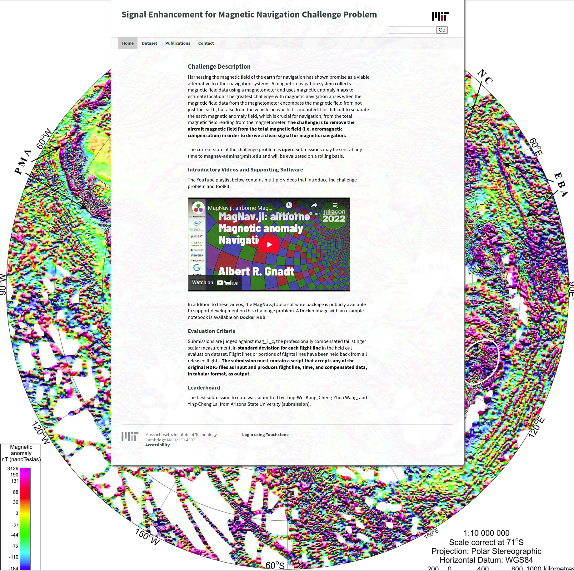
Software and Data for Tutorial
MIT-AF AI Accelerator MagNav project
Collected data and made publicly available:
Created software suite published on GitHub:
- Written in Julia https://juilalang.org
- https://github.com/MIT-AI-Accelerator/MagNav.jl
- Docker container https://hub.docker.com/r/jtaylormit/magnav
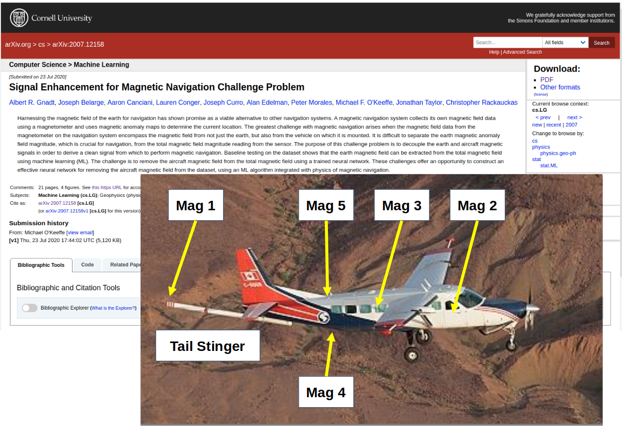
Data run-thru
- Collected data made publicly available:
- https://zenodo.org/record/6327685
- Hold-out data for challenge problem
- Recorded flight data near Ottawa, ON
- Position, velocity, attitude (truth)
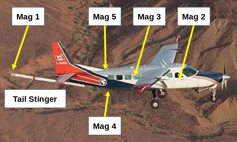
- Tail Stinger
- 4 magnetometers in cabin
- Current and voltage sensors
- 10 Hz
- Ground station reference sensor
- 10 Hz
- Magnetic Maps of flight area
- Calibration maneuvers
- Flight crew notes
- Power lines
- Railroad tracks
- On-board activities
- power on/off to systems
- movement of iron bars
- Professional calibration results
MagNav Software - MagNav.jl
https://github.com/MIT-AI-Accelerator/MagNav.jl

MagNav.jl Docker image
https://hub.docker.com/r/jtaylormit/magnav

Challenge problem
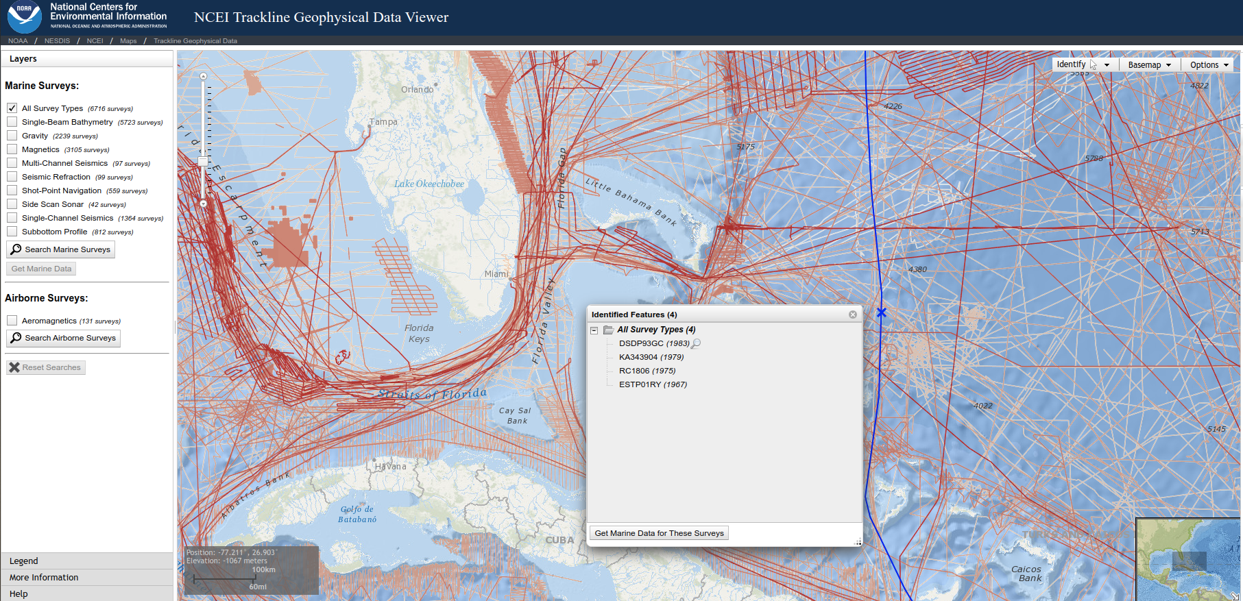
Airborne magnetic anomaly surveys
- Usually performed in smaller area for geological interpretation
- Large anomaly maps merged together in mosaic using a leveling process
- Meant to merge long spatial wavelengths
- Many anomaly surveys pre-date GPS
- Geolocated via air-crew observations
- Typically remove space-weather effects with ground-station
Marine track surveys
- Often single long track following ship
- Many pre-date GPS
- Use ship’s positioning
- Typically no space weather correction
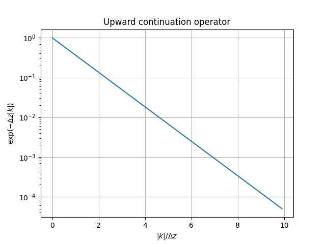
Upward continuation
Magnetic anomaly maps are usually made at a single altitude.
The process of taking a magnetic map from one altitude to another.
- \(F(B_\text{up}) = F(B_\text{known}) e^{-\Delta z |k|}\)
- Assumes a flat Earth model with all the sources below
- (Blakely 1995)
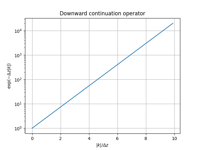
Dangerous downward continuation
The process of taking a magnetic map from one altitude to another.
- \(F(B_\text{down}) = F(B_\text{known}) e^{+\Delta z |k|}\)
- Noise can be amplified
- Techniques to do this exist, and involve some kind of regularization or source estimation
- (Blakely 1995)
Tolles-Lawson
- Calibration technique developed in WW2 for submarine hunting
- Declassified in 1950’s and patented
- Standard calibration technique used for aero-magnetic surveys
- Developed by (Leliak 1961)
\[ \begin{align*} |B_\mathrm{Sensor}| &= |\vec{B}_\ext + \vec{B}_\faPlane|\\ &= \sqrt{ |B_\ext|^2 + |B_\faPlane|^2 + 2 |B_\ext||B_\faPlane|\cos\theta}\\ |B_\text{Sensor}| &= |B_\ext| \sqrt{ 1 + \frac{|B_\faPlane|^2}{|B_\ext|^2} + 2\frac{|B_\faPlane|}{|B_\ext|}\cos\theta} \end{align*} \]
Tolles-Lawson Path to Calibration 1/2
\[
\begin{align*}
|B_\text{Sensor}| &= |\vec{B}_\ext + \vec{B}_\faPlane|\\
&= \sqrt{ |B_\ext|^2 + |B_\faPlane|^2 + 2 |B_\ext||B_\faPlane|\cos\theta}\\
|B_\text{Sensor}| &= |B_\ext| \sqrt{ 1 + 2\frac{|B_\faPlane|}{|B_\ext|}\cos\theta}\\
&\approx |B_\ext| + |B_\faPlane|\cos\theta + \cdots
\end{align*}
\]
Path to Calibration
Measure \(\cos\theta\)
Solve \(|B_\text{sensor}| = |B_\ext| + |B_\plane|\cos\theta\)
Assuming \(|B_\ext|\) is known or constant
Tolles-Lawson Path to Calibration 2/2

Path to Calibration
Measure \(\cos\theta\)
Solve \(|B_\text{sensor}| = |B_\ext| + |B_\faPlane|\cos\theta\)
Assuming \(|B_\ext|\) is known or constant
How to measure \(\cos\theta\)?
Use a vector magnetometer
Rotate aircraft in \(|B_\ext|\)
Compute direction cosines…
Calibration 1/4
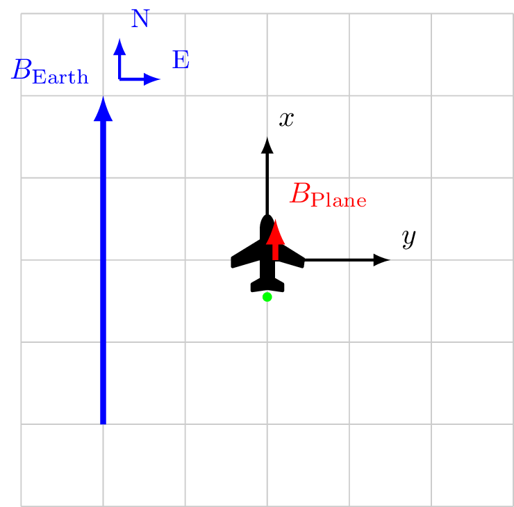
Coordinate system fixed to aircraft
\[\vec{B}_\mathrm{Sensor} = \vec{B}_\ext + \vec{B}_\faPlane\]
\[
\begin{alignat*}{3}
\vec{B}_\ext &= 4.0 \hat{x} && + 0.0 \hat{y} \\
\vec{B}_\faPlane &= 0.5 \hat{x} && +0.0 \hat{y} \\
\vec{B}_\text{Sensor} &= 4.5 \hat{x} && + 0.0 \hat{y} \\
|B_\text{Sensor}| &= 4.5 && \\
\cos X &= \frac{4.5}{4.5} && = 1\\
\cos Y &= \frac{0.0}{4.5} && = 0\\
\end{alignat*}
\]
Calibration 2/4
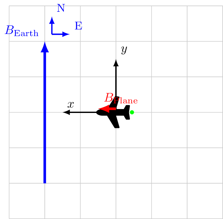
Coordinate system fixed to aircraft
\[\vec{B}_\text{Sensor} = \vec{B}_\ext + \vec{B}_\faPlane\]
\[
\begin{alignat*}{3}
\vec{B}_\ext &= 0.0 \hat{x} && + 4.0 \hat{y} \\
\vec{B}_\faPlane &= 0.5 \hat{x} && + 0.0 \hat{y} \\
\vec{B}_\text{Sensor} &= 0.5 \hat{x} && + 4.0 \hat{y} \\
|B_\text{Sensor}| &= 4.007 && \\
\cos X &= \frac{0.5}{4.007} && \ne 0 \rightarrow 82.8^\circ\\
\cos Y &= \frac{4.0}{4.007} && \approx 1\\
\end{alignat*}
\]
Calibration 3/4
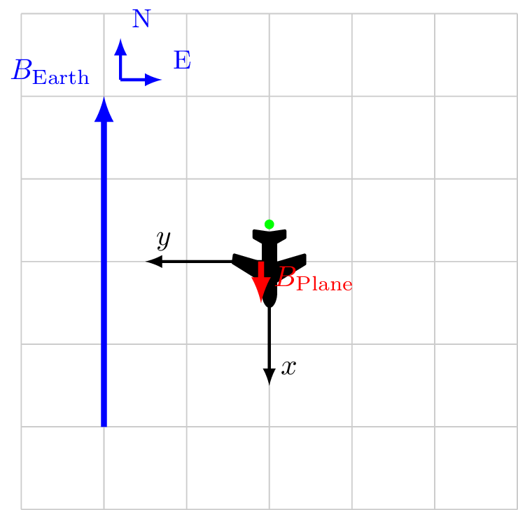
Coordinate system fixed to aircraft
\[\vec{B}_\text{Sensor} = \vec{B}_\ext + \vec{B}_\faPlane\]
\[
\begin{alignat*}{3}
\vec{B}_\ext &= -4.0 \hat{x} && + 0.0 \hat{y} \\
\vec{B}_\faPlane &= 0.5 \hat{x} && + 0.0 \hat{y} \\
\vec{B}_\text{Sensor} &= -3.5 \hat{x} && + 0.0 \hat{y} \\
|B_\text{Sensor}| &= 3.5 && \\
\cos X &= \frac{-3.5}{3.5} && = -1\\
\cos Y &= \frac{0}{3.5} && = 0\\
\end{alignat*}
\]
Calibration 4/4
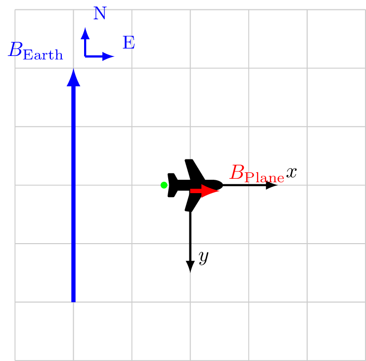
Coordinate system fixed to aircraft
\[\vec{B}_\text{Sensor} = \vec{B}_\ext + \vec{B}_\faPlane\]
\[
\begin{alignat*}{3}
\vec{B}_\ext &= 0.0 \hat{x} && + -4.0 \hat{y} \\
\vec{B}_\faPlane &= 0.5 \hat{x} && + 0.0 \hat{y} \\
\vec{B}_\text{Sensor} &= 0.5 \hat{x} && + -4.0 \hat{y} \\
|B_\text{Sensor}| &= 4.007 &&\\
\cos X &= \frac{0.5}{4.007} && \ne 0\\
\cos Y &= \frac{-4.0}{4.007} && \approx -1\\
\end{alignat*}
\]
Standard calibration model
\[|\vec{B}| = |\vec{B}_\ext + \vec{B}_\faPlane|\]
\[ \begin{array}{ l B c B c B c } \vec{B}_\faPlane & = & \vec{B}_\text{Permanent} & + & \vec{B}_\text{Induced} & + & \vec{B}_\text{Eddy}\\ & = & \vec{P}_\text{constant} {} & + &{} M_{3\times3} \vec{B }_\ext {} & + & {} S_{3\times3} \frac{\partial}{\partial t} \vec{B}_\ext \end{array} \]
\(M_{3\times3}\) is symmetric \(\rightarrow\) 6 independent elements
Total of 18 elements

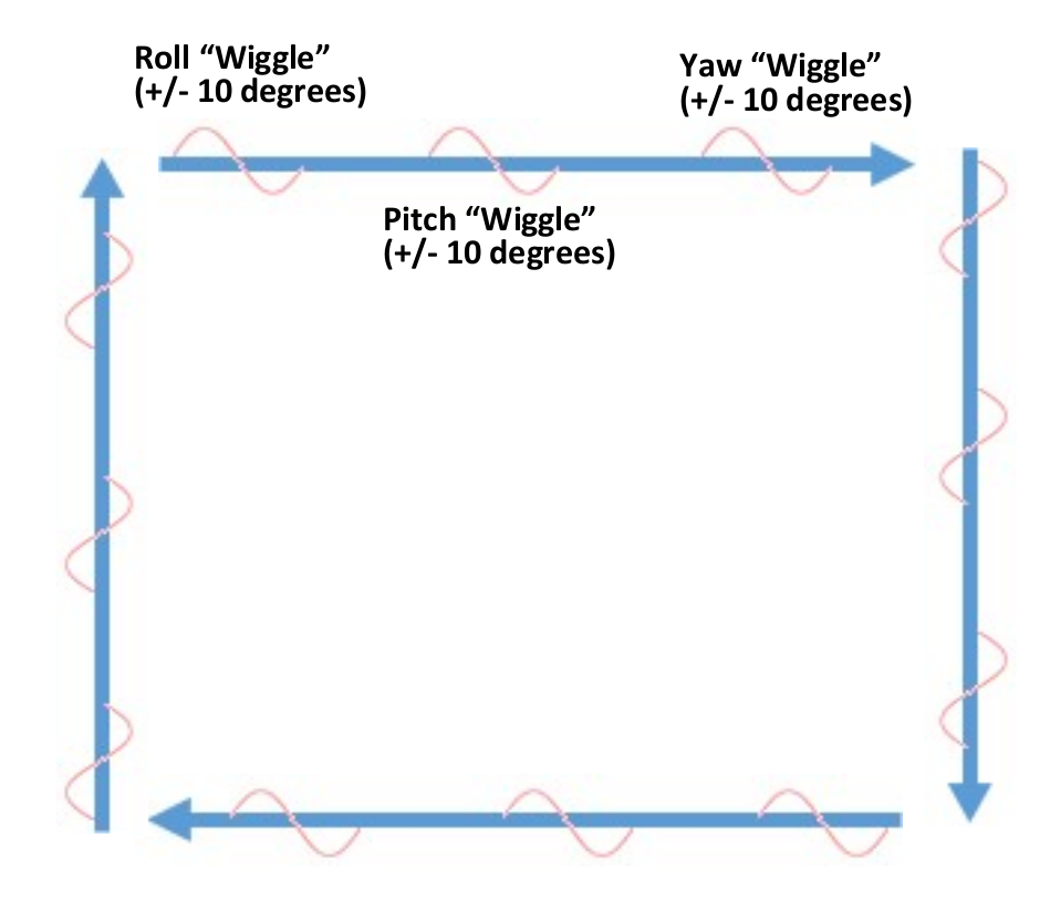
Calibration manuevers - Tolles-Lawson
Fly the aircraft in a series of Roll, Pitch, Yaw maneuvers
High-altitude
Altitude of a known map
Maneuver angle should depend upon the expected aircraft dynamics
- Barrel Rolls?
Typically at each cardinal heading
- 3 rolls \(\pm 10^\circ\) at 1 Hz
- 3 pitches \(\pm 10^\circ\) at 1 Hz
- 3 yaws \(\pm 10^\circ\) at 1 Hz
Pack your air-sickness bag
(W. E. Tolles and Lawson 1950), (W. E. Tolles 1954), (W. E. Tolles 1955), (Gnadt, Wollaber, and Nielsen 2022)
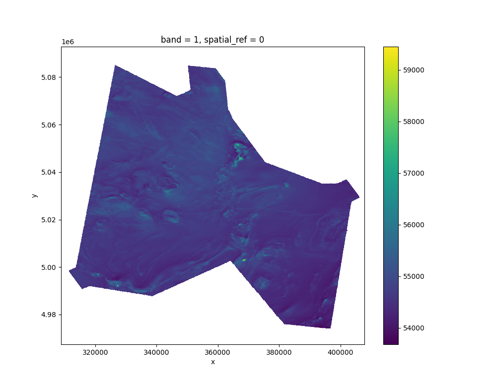
Load a magnetic anomaly map and plot it

Plot the GPS flight trajectory with map


Plot calibration trajectory data


How good is the professional calibration?

Plot scalar magnetometers during T-L manuevers

Plot scalar magnetometers during T-L manuevers

Plot scalar mags during T-L manuevers (detrend)

Plot vector magnetometers during T-L manuevers

Look at compensation results
Applied to the compensation data
Magnetometer 4 300 nT/division


Plot compensation results on flight data
Magnetometer 4 300 nT/division
Code
p = plot(
     traj_flt.tt[ind],
     mag_4_uc,
     xlabel="Time [seconds]",
     ylabel="Magetic intensity [nT]",
     legend=true,
     label="Uncomp Mag 4",
     linecolor=:green
);
plot!(
     traj_flt.tt[ind],
     mag_4_c,
     label="Comp Mag 4",
     linecolor=:black
)
plot!(
     traj_flt.tt[ind],
     mag_1_sgl,
     label="Comp tail Stinger",
     linecolor=:red
)
plot!(p; double_pane_defs...)
Magnetometer 5 100 nT/division
Code
p = plot(
     traj_flt.tt[ind],
     mag_5_uc,
     xlabel="Time [seconds]",
     ylabel="Magetic intensity [nT]",
     legend=true,
     label="Uncomp Mag 5",
     linecolor=:green
);
plot!(
     traj_flt.tt[ind],
     mag_5_c,
     label="Comp Mag 5",
     linecolor=:black
)
plot!(
     traj_flt.tt[ind],
     mag_1_sgl,
     label="Comp tail Stinger",
     linecolor=:red
)
plot!(p; double_pane_defs...)
Compare to professional calibration
Magnetometer 4
Code
p = plot(
     traj_flt.tt[ind],
     detrend(mag_4_c-mag_1_sgl;mean_only=true),
     xlabel="Time [seconds]",
     ylabel="Magnetic intensity [nT]",
     legend=true,
     linecolor=:black,
     label="Comp 4 - Comp Stinger"
)
plot!(
     traj_flt.tt[ind],
     detrend(mag_4_uc-mag_1_sgl;mean_only=true),
     linecolor=:green,
     label="Uncomp 4 - Comp Stinger"
)
plot!(p; double_pane_defs...)
Magnetometer 5
Code
p = plot(
     traj_flt.tt[ind],
     detrend(mag_5_c-mag_1_sgl;mean_only=true),
     xlabel="Time [seconds]",
     ylabel="Magnetic intensity [nT]",
     legend=true,
     linecolor=:black,
     label="Comp 5 - Comp Stinger"
)
plot!(
     traj_flt.tt[ind],
     detrend(mag_5_uc-mag_1_sgl;mean_only=true),
     linecolor=:green,
     label="Uncomp 5 - Comp Stinger"
)
plot!(p; double_pane_defs...)
Compare to professional calibration
Magnetometer 4
Code

Magnetometer 5
Code

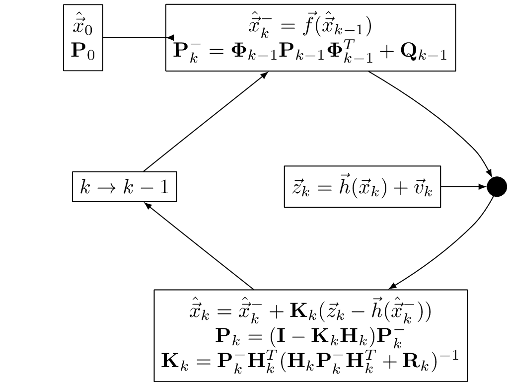
Kalman filter flow diagram
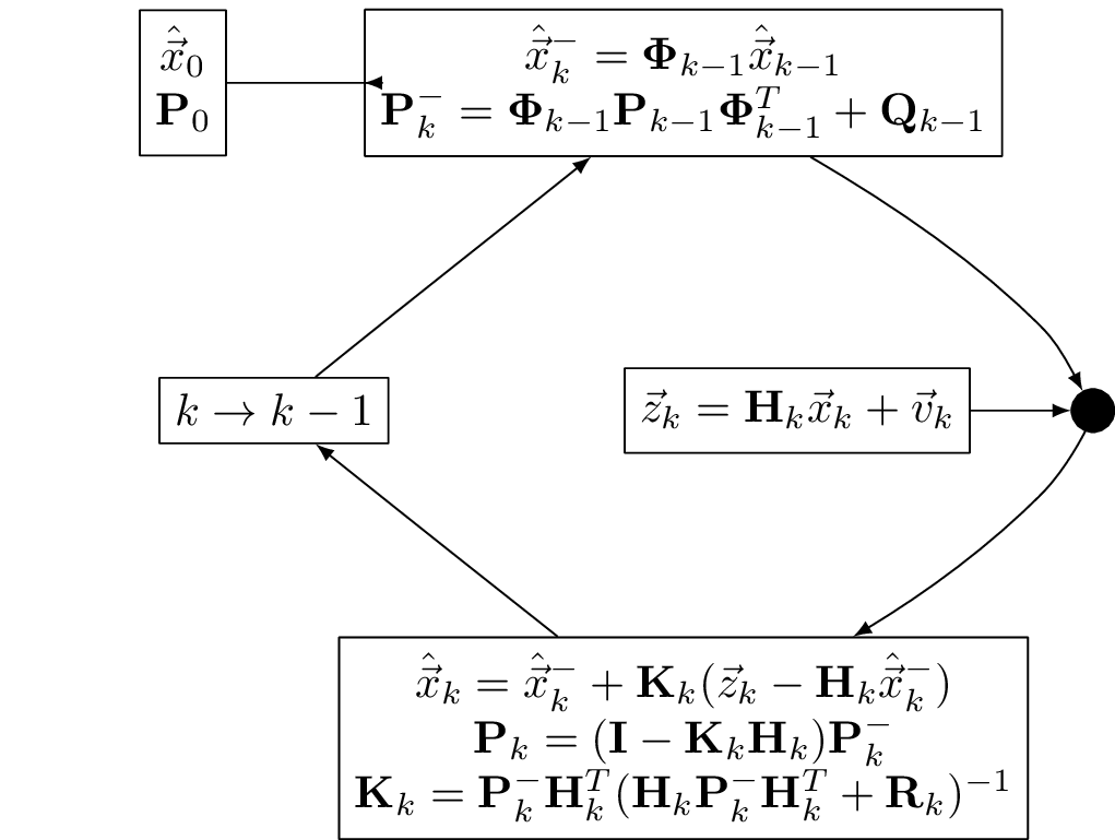
EKF data flow
Plot navigation trajectory (GPS)
Entire map


Plot navigation trajectory (GPS and INS)
Entire map

Zoom on selected flight line
Code

GPS track
INS only
Notice overall shift between tracks
Set up data for navigation
Uncorrected GPS and INS tracks
Code

\(\rightarrow\)
Shifted GPS and INS tracks

Upward continue and prepare map


Compare map value with magnetometer values


Create EKF filter model
FOGM filter tuning parameters

EKF filter generation
Run the filter
Mag 4 DRMS Error = 149.2 meter
Mag 5 DRMS Error = 82.5 meter
INS DRMS Error = 137.5 meter
North position error
Code
tt_min = (traj.tt .- traj.tt[1])./60;
p=error_plot(tt_min,filt_out_4.n_err,filt_out_4.n_std, color=:blue, label="Mag 4, North error",xlabel="Time [minutes]", ylabel="North Error [meters]")
error_plot(p,tt_min,filt_out_5.n_err,filt_out_5.n_std, color=:green,label="Mag 5, North error",xlabel="Time [minutes]", ylabel="North Error [meters]")
plot(p; double_pane_defs...)
East position error
Code
p=error_plot(tt_min,filt_out_4.e_err,filt_out_4.e_std, color=:blue, label="Mag 4, East error",xlabel="Time [minutes]", ylabel="East Error [meters]")
error_plot(p,tt_min,filt_out_5.e_err,filt_out_5.e_std, color=:green, label="Mag 5, East error",xlabel="Time [minutes]", ylabel="East Error [meters]")
plot(p; double_pane_defs...)
Inertial only solution


Plot filter results

Scalar Potential Theory
A procedure to transform magnetic scalar potential \(\Phi_M\) in free space.
From Laplacian we can write (Green’s third identity) \[
\Phi_M(\vec{r}) = \frac{1}{4\pi} \int_S \left( \frac{1}{r} \frac{\partial \Phi_M}{\partial n} -
\Phi_M \frac{\partial}{\partial n} \frac{1}{r} \right) dS
\]
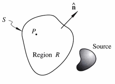
- No sources in region \(R\)
- Know \(\Phi_M\) on the surface \(S\) that bounds \(R\)
- We can find \(\Phi_M\) anywhere in \(R\)
- (Blakely 1995)
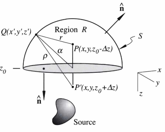
Hemispherical geometry - flat Earth model
- Think of Earth’s surface as an infinite flat plane, all sources below
- Measure the potential on a plane above the earth
- Other side of hemisphere is \(\infty\) away and therefore zero potential
- Potential anywhere inside can be computed
Fourier methods for potential theory
- Goal: find the potential \(\Phi_M\) on a plane parallel to a known plane
- Process: double integral over the surface of the known plane
- Ends up looking like a 2-D Fourier transform over spatial coordinates
- (Blakely 1995)

Bankey, Viki, Alejandro Cuevas, David Daniels, Carol A. Finn, Israel Hernandez, Patricia Hill, Robert Kucks, et al. 2002. “Digital Data Grids for the Magnetic Anomaly Map of North America.” U.S. Department of the Interior, U.S. Geological Survey; Online; US Geological Survey. https://doi.org/10.3133/ofr02414.
Blakely, Richard J. 1995. Potential Theory in Gravity and Magnetic Applications. Cambridge University Press.
Brown, Robert Grover, and Patrick Y C Hwang. 2012. Introduction to random signals and applied kalman filtering: with MATLAB exercises and solutions; 4th ed. New York, NY: Wiley.
Canciani, Aaron J. 2016. “Absolute Positioning Using the Earth’s Magnetic Field.” PhD thesis, Air Force Institute of Technology. https://scholar.afit.edu/etd/251.
———. 2021. “Magnetic Navigation on an f-16 Aircraft Using Online Calibration.” IEEE Trans. Aerospace and Electronic Systems. https://doi.org/10.1109/TAES.2021.3101567.
Chulliat, A.;W. Brown;P. Alken;C. Beggan;M. Nair;G. Cox;A. Woods;S. Macmillan;B. Meyer;M. Paniccia; 2020. “The US/UK World Magnetic Model for 2020-2025 : Technical Report.” National Centers for Environmental Information (U.S.);British Geological Survey. https://doi.org/10.25923/ytk1-yx35.
Clarke, Daniel J. 2021. “Real-Time Aerial Magnetic and Vision-Aided Navigation.” Master’s thesis, Air Force Institute of Technology. https://scholar.afit.edu/etd/4994/.
Gelb, Arthur et al. 1974. Applied Optimal Estimation. MIT press.
Gnadt, Albert R., Joeseph Belarge, Aaron Cancini, Lauren Conger, Joseph Curro, Alan Edelman, Peter Morales, Michael O’Keefe, Jonathan Taylor, and Chrstopher Rackaukas. 2020. “Signal Enhancement for Magnetic Navigation Challenge Problem,” July. https://doi.org/10.48550/ARXIV.2007.12158.
Gnadt, Albert R., Allan B. Wollaber, and Aaron P. Nielsen. 2022. “Derivation and Extensions of the Tolles-Lawson Model for Aeromagnetic Compensation.” arXiv. https://doi.org/10.48550/ARXIV.2212.09899.
Leliak, Paul. 1961. “Identification and Evaluation of Magnetic-Field Sources of Magnetic Airborne Detector Equipped Aircraft.” IRE Transactions on Aeronautical and Navigational Electronics ANE-8 (3): 95–105. https://doi.org/10.1109/TANE3.1961.4201799.
McNeil, Alexander J. 2022. “Magnetic Anomaly Absolute Positioning for Hypersonic Aircraft.” Master’s thesis, Air Force Institute of Technology. https://scholar.afit.edu/etd/5457.
Meyer, B., A. Chulliat, and R. Saltus. 2017. “Derivation and Error Analysis of the Earth Magnetic Anomaly Grid at 2 Arc Min Resolution Version 3 (EMAG2v3).” Geochemistry, Geophysics, Geosystems 18 (12): 4522–37. https://doi.org/10.1002/2017gc007280.
Mount, Lauren A. 2018. “Navigation Using Vector and Tensor Measurements of the Earth’s Magnetic Anomaly Field.” Master’s thesis, Air Force Institute of Technology. https://scholar.afit.edu/etd/1817/.
Raquet, John. 2021. “Pinson 15 Model.”
Roberts, Carter W., and Robert C. Jachens. 2000. “Preliminary Aeromagnetic Anomaly Map of California.” United States Geologic Survey. https://pubs.usgs.gov/of/1999/0440/.
Titterton, David, and John Weston. 2004. Strapdown Inertial Navigation Technology. Institution of Engineering; Technology. https://doi.org/dx.doi.org/10.1049/PBRA017E.
Tolles, W E, and J D Lawson. 1950. “Magnetic compensation of MAD equipped aircraft.” Airborne Instruments Lab. Inc., Mineola, NY, Rept, 201–1.
Tolles, W. E. 1954. Compensation of aircraft magnetic fields. 2692970, issued 1954.
———. 1955. Magnetic field compensation system. 2706801, issued 1955.