
Workshop Presentation Materials
ION MagNav Workshop 2023, Monterey, CA
The views expressed in this article are those of the author and do not necessarily reflect the official policy or position of the United States Government, Department of Defense, United States Air Force or Air University.
Distribution A: Authorized for public release. Distribution is unlimited. Case No. 2023-0427.
Introduction
https://rpubs.com/friendly/test-newcommands https://quarto.org/docs/authoring/markdown-basics.html#equations
https://stackoverflow.com/questions/41362012/how-to-insert-font-awesome-icons-in-mathjax
Font-Awesome will only work for html type output
$$$$
Background and Problem description
- Magnetic anomaly navigation (MagNav) overview
Magnetic Anomaly Navigation Overview
https://rpubs.com/friendly/test-newcommands https://quarto.org/docs/authoring/markdown-basics.html#equations
https://stackoverflow.com/questions/41362012/how-to-insert-font-awesome-icons-in-mathjax
Font-Awesome will only work for html type output
$$$$
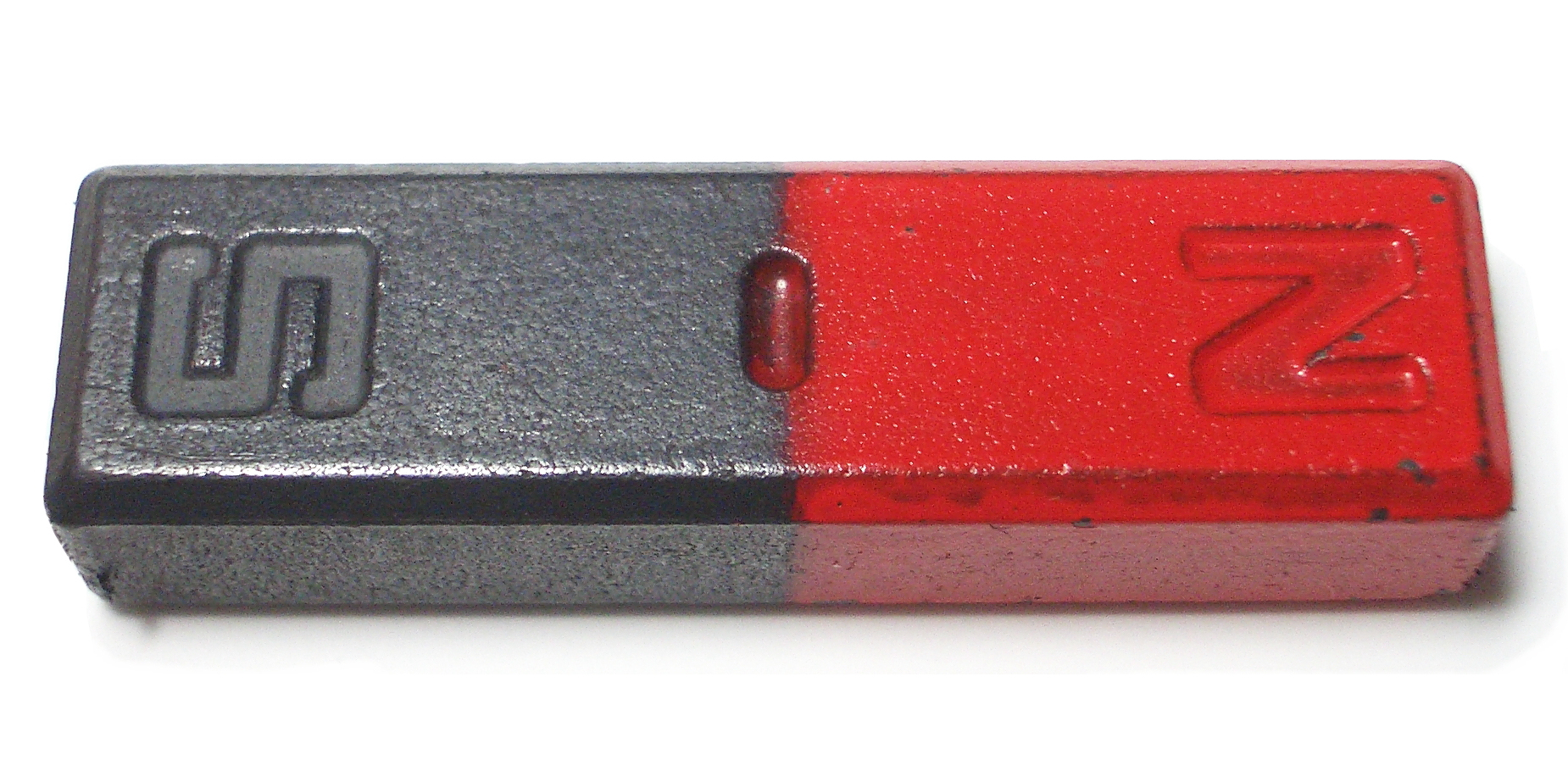
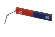
Refrigerator magnet 
Earth’s core field (compass) 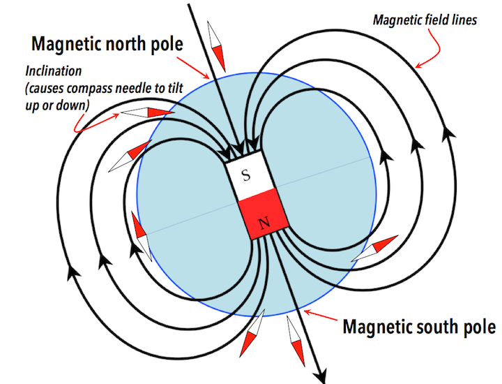
Crustal magnetic anomaly 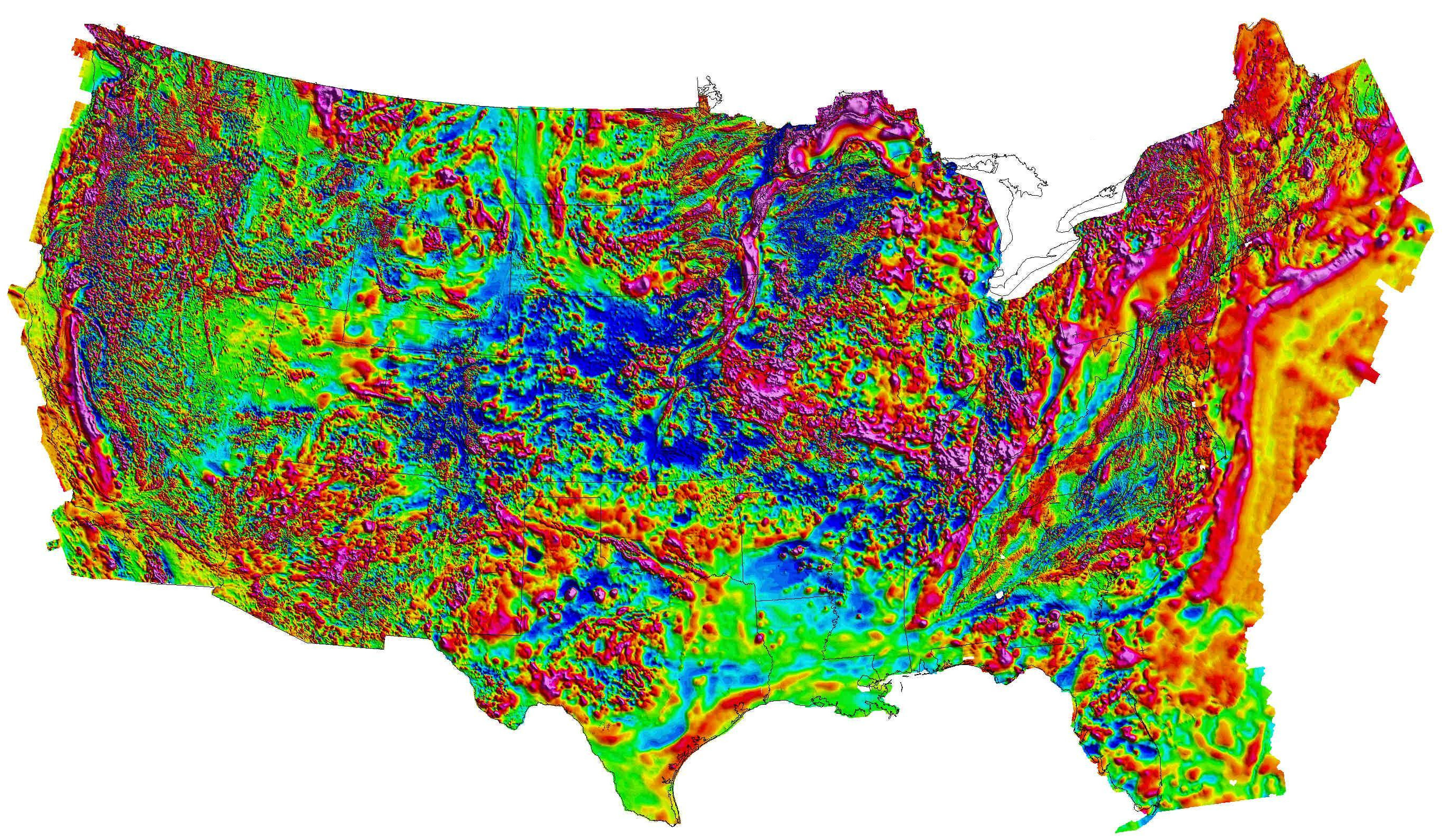
1 000 000 nT
Range \(\pm\) 500 nT
Resolution \(\sim\) 1 nT https://mrdata.usgs.gov/magnetic/ (Bankey et al. 2002)
Requirements for MagNav
- Maps
- Sensors
- Platform Calibration
- Navigation Algorithms
Maps
Map-based navigation
- Features are required to navigate
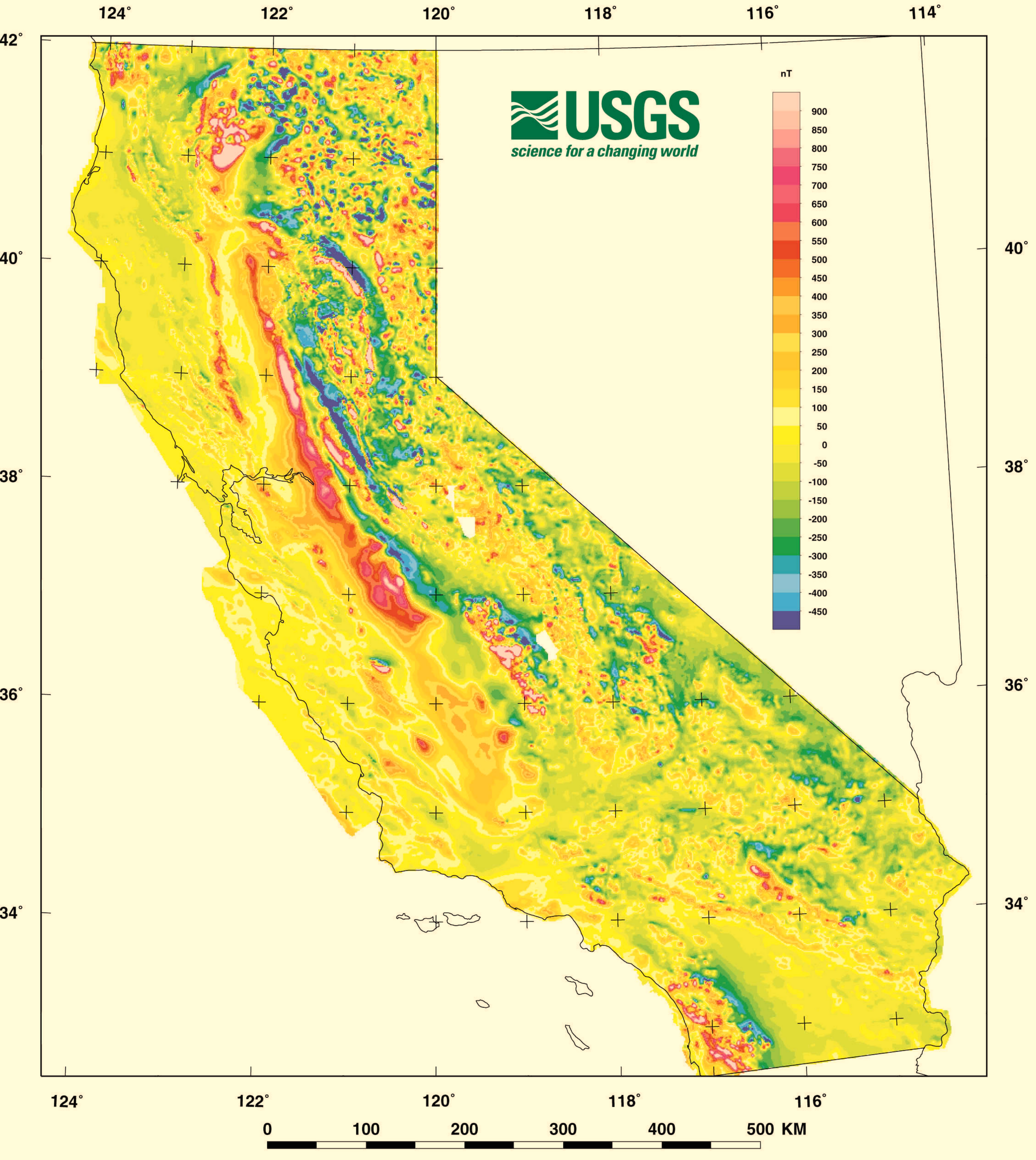
- Magnetic anomaly closely tied to geology
- less variation in coastal region
- direction variation in Central Valley
- more structure in Sierra Nevada mountains
- Area and direction of travel make a difference
(Roberts and Jachens 2000)
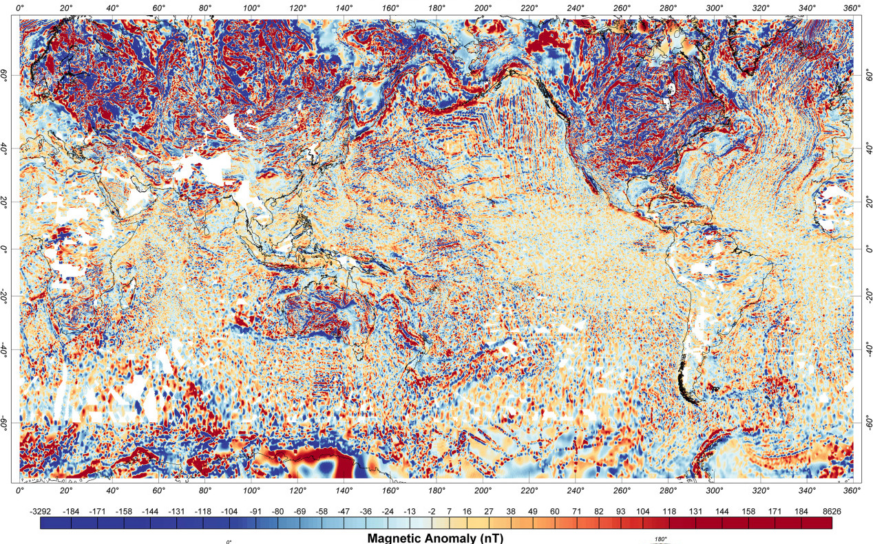
Map coverage required - Earth Magnetic Anomaly Grid 2-arcsec v3
Sensors
Sensors
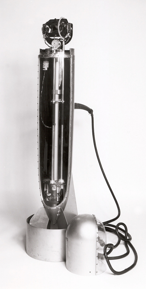
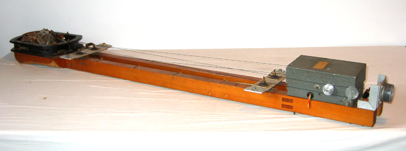
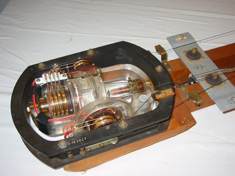
Vaquier towed magnetometer, National Museum of American History (Smithsonian Institution, n.d.) Ca. 1946
Platform calibration
An airplane is a big magnet that flies
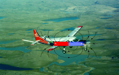
\(|\vec{B}_\text{sensor}| = |\vec{B}_{\oplus}+ \vec{B}_\text{anomaly}+ \vec{B}_\class{fa fa-plane}{}|\)
Aircraft Calibration
Sensor placement and installation
- Engineered location
- Stinger
- Survey for placement
- Non-magnetic fasteners
Degaussing
Algorithms
Navigation algorithms
Navigation algorithms
Inertial navigation aiding
Map-matching
- Kalman filter
- contour matching/Correlation processing
Inertial Navigation
- Inertial Measurement Unit (IMU)
- measures accelerations \(\vec{f}\)
- measures rotation rates \(\dot{\vec{\theta}}\)
- To get position from accleration, you have to integrate twice
- continuously adds noise to your position estimate
- Drifting position estimate needs to be corrected
- MagNav!
Map matching
- Sequential measurement Kalman filtering
- Contour matching/Correlation processing
Magnetics
Magnetics
- Derivations
- Maxwell’s equations \(\rightarrow\) Quasi-magnetostatics
- Magnetic dipoles
- Magnetic fields in free space
- Terminology and definitions
- Textbooks and literature are not consistent
From electromagnetics
Maxwell’s equations in MKS units (Griffiths 1999)
\(\nabla \cdot \vec{B} = 0\)
\(\nabla \times \vec{H} = \vec{J} + \frac{\partial \vec{D}}{\partial t}\)
\(\nabla \cdot \vec{D} = \rho\)
\(\nabla \times \vec{E} = -\frac{\partial \vec{B}}{\partial t}\)
Constituent relationships apply in a physical medium
\(\vec{B} = \mu_0 \left(\vec{H} + \vec{M} \right)\)
Ohm’s law \(\vec{J} = \sigma \vec{E}\)
\(\vec{E} = \frac{1}{\epsilon_0} \left( \vec{D} - \vec{P} \right)\)
To quasi-magnetostatics
\[ \frac{\partial \vec{E}}{\partial t} \approx \frac{\partial \vec{D}}{\partial t} \approx 0, \rho = 0 \]
\(\nabla \cdot \vec{B} = 0\)
\(\nabla \times \vec{H} = \vec{J} + \cancelto{0}{\frac{\partial \vec{D}}{\partial t}}\)
\({\nabla \cdot \vec{D} = \cancelto{0}{\rho}}\)
\({\nabla \times \vec{E} = -\frac{\partial \vec{B}}{\partial t}}\)
\(\vec{B} = \mu_0 \left(\vec{H} + \vec{M} \right)\)
Ohm’s law \(\vec{J} = \sigma \vec{E}\)
\({\vec{E} = \frac{1}{\epsilon_0} \left( \vec{D} - \cancelto{0}{\vec{P}} \right)}\)
Quasi-magnetostatic limits
How do we know that we can use quasi-magnetostatics? (Bulovic et al. 2011)
Want the error \(\frac{H_\mathrm{error}}{H} \rightarrow 0\) in neglecting \(\frac{\partial \vec{D}}{\partial t}\)
Via Stokes’ Theorem \[\oint_C \vec{H}_{\mathrm{error}} \cdot d\ell = \int_S \frac{\partial \vec{D}}{\partial t} da
\] with \[
\vec{D} = \epsilon_0 \vec{E} e^{-i \omega t}
\] and characteristic length scale \(L\) then \[
H_{\mathrm{error}} L = i \epsilon_0 \omega E L^2
\]
Quasi-magnetostatic \(H\)
\[ {\nabla \times \vec{E} = -\frac{\partial \vec{B}}{\partial t}} \] Similar to before from Stokes’ Theorem \[ \oint \vec{E} \cdot d \ell = - \frac{\partial }{\partial t} \int_S \vec{H} \cdot d\vec{a} \] similar hand-waving \[ EL = -i \omega \mu_0 H L^2 \] and then \[ \frac{H_\mathrm{error}}{H} = \omega^2 {\mu_0 \epsilon_0} L^2 = \frac{\omega^2 L^2 }{c^2} = \frac{L^2}{\lambda^2} \] assuming free space: \(\mu = \mu_0\) and \(\epsilon = \epsilon_0\)
Quasi-magnetostatic limit applicability
\[ \frac{H_\mathrm{error}}{H} = \omega^2 {\mu_0 \epsilon_0} L^2 = \frac{\omega^2 L^2 }{c^2} = \frac{L^2}{\lambda^2} \]
#| echo: false
#| output: true
import numpy as np
from scipy.constants import speed_of_light as c

from matplotlib import pylab as plt
plt.ion()

freqs = np.array([0.1, 1, 10, 100])

wavelens = c/freqs

fg,ax = plt.subplots()
ax.loglog(freqs,wavelens,label='Wavelength')
ax.grid()
ax.set_xlabel('Frequency [Hertz]')
ax.set_ylabel('Wavelength [meter]')
ax.hlines(y=12.742e6,xmin=freqs[0], xmax=freqs[-1],color='red',label='Earth diameter')
ax.hlines(y=384.4e6,xmin=freqs[0], xmax=freqs[-1],color='green',label='Earth-moon distance')
_ = ax.legend()
World’s largest container ship, 400 m long.
Quasi-magnetic limit failure
Speed of light in sea-water (Moser 1989), (Hunt, Niemeier, and Kruger 2010) \[v \approx 2 \sqrt{\frac{\pi \nu}{\mu_0 \sigma}}\]
#| echo: false
seawater_conductivity = 4.5 # 3-6 S/m
seawater_permeability = 4*np.pi*1e-7 # H/m
vel = 2*np.sqrt(np.pi*freqs/seawater_permeability/seawater_conductivity)

fg,ax = plt.subplots()
ax.loglog(freqs,vel,)
ax.grid()
ax.set_xlabel('Frequency [Hertz]')
ax.set_ylabel('Velocity [meters/second]')
_ = ax.set_title('Speed of light in seawater')
#| echo: false
fg,ax = plt.subplots()
ax.loglog(freqs,vel/freqs)
ax.grid()
ax.set_xlabel('Frequency [Hertz]')
ax.set_ylabel('Wavelength [meters]')
ax.set_title('Wavelength in seawater')
ax.hlines(y=400,xmin=freqs[0], xmax=freqs[-1],color='red',label='Container ship')
ax.hlines(y=1,xmin=freqs[0], xmax=freqs[-1],color='green',label='1 meter')
_ = ax.legend()Dipoles
Magnetic potentials
Vector Potential \(\vec{A}\)
\(\vec{B}(\vec{r}) = \nabla \times \vec{A}(\vec{r})\)
General case
Will use to discuss dipoles today
Scalar Magnetic Potential \(\Phi_M\)
- If \(\vec{J} = 0\), then \(\nabla \times \vec{H} = 0\)
- \(\vec{H}(\vec{r}) = -\nabla \Phi_M(\vec{r})\)
- This situation holds for many airborne problems
Vector potential
Magnetic field is divergence free: \[ \nabla \cdot \vec{B} = 0 \] There’s a vector identity: \[ \nabla \cdot (\nabla \times \vec{F} ) = 0 \] So \(\vec{B}\) can be expressed as a curl \[ \vec{B} = \nabla \times \vec{A} \] Subsittute into Ampere’s law \[ \nabla \times \vec{H} = \mu_0 \vec{J} = \nabla \times (\nabla \times \vec{A}) = \nabla(\nabla\cdot\vec{A}) - \nabla^2 \vec{A} \] \(\vec{A}\) is not unique for a given \(\vec{B}\).
Vector potential continued
\(\vec{A}\) is not unique for a given \(\vec{B}\) \[ \vec{A} \rightarrow \vec{A} + \nabla f \] from vector identity \[ \nabla \times \nabla f = 0 \] A unique \(\vec{B}\) will exist \[ \vec{B} = \nabla \times \vec{A} = \nabla \times ( \vec{A} + \nabla f) \] We can choose some \(f\) so that \(\nabla \cdot \vec{A} = 0\) which results in \[ \nabla^2 \vec{A} = - \mu_0 \vec{J} \ \mathrm{,Poisson's\ Equation} \] Which has solution \[ \vec{A}(\vec{r}) = \frac{\mu_0}{4\pi} \int \frac{\vec{J}(\vec{r}') }{ \left| \vec{r} - \vec{r}' \right| } d^3 r' \]
Multipole expansion
To find the equation of a dipole (Griffiths 1999) \[ \vec{A}(\vec{r}) = \frac{\mu_0}{4\pi} \int \frac{\vec{J}(\vec{r}')}{ \left| \vec{r} - \vec{r}' \right| } d^3 r' \] \[ \begin{align*} \frac{1}{\left| \vec{r} - \vec{r}' \right| } &= \frac{1}{\sqrt{r^2 + (r')^2 - 2 r r' cos\theta'}} \\ &= \frac{1}{r} \sum_{n=0}^{\infty} \left( \frac{r'}{r} \right)^n P_n(\cos\theta') \end{align*} \] \[ \vec{A}(\vec{r}) = \frac{\mu_0 I}{4\pi} \left[ \cancelto{0}{\frac{1}{r} \oint d\vec{\ell}' } + \frac{1}{r^2} \oint r' \cos\theta' d \vec{\ell}' + \frac{1}{r^3} \oint (r')^2 \left( \frac{3}{2} \cos^2 \theta' -\frac{1}{2} \right) d \vec{\ell}' \cdots \right] \]
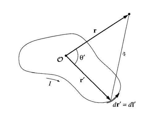
Monopoles, dipoles and quadrapoles
\[ \vec{A}(\vec{r}) = \frac{\mu_0 I}{4\pi} \left[ \cancelto{0}{\frac{1}{r} \oint d\vec{\ell}' } + \frac{1}{r^2} \oint r' \cos\theta' d \vec{\ell}' + \frac{1}{r^3} \oint (r')^2 \left( \frac{3}{2} \cos^2 \theta' -\frac{1}{2} \right) d \vec{\ell}' \cdots \right] \]
Monopole
There are no magnetic monopoles \(\nabla\cdot\vec{B}=0\)
Dipole

Quadrapole

Dipole derivation
\[ \vec{A}_\mathrm{dipole}(\vec{r}) = \frac{\mu_0 I}{4\pi} \left[ \frac{1}{r^2} \oint r' \cos\theta' d \vec{\ell}' \right] \] some more vector trickery \[ \vec{A}_\mathrm{dipole}(\vec{r}) = \frac{\mu_0 }{4\pi} \frac{\vec{m} \times \hat{r}}{r^2} \] where magnetic moment is defined as \[ \vec{m} = I \int d\vec{a} = I\vec{a} \] Finally from \(\vec{B} = \nabla \times \vec{A}\) \[ \vec{B}_\mathrm{dipole} = \frac{\mu_0 }{4\pi} \frac{1}{r^3} \left[ 3 (\vec{m}\cdot \hat{r})\hat{r} - \vec{m} \right] \]
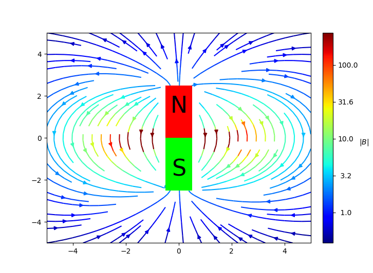
Dipole field lines
\[
\vec{B}_\mathrm{dipole} = \frac{\mu_0 }{4\pi} { \frac{1}{r^3} }\left[ 3 (\vec{m}\cdot \hat{r})\hat{r} - \vec{m} \right] \propto \frac{1}{r^3}
\tag{1}\]
Inverse cube dependence on distance from dipole \({ \frac{1}{r^3} }\)

Physically large dipole - Bar magnet
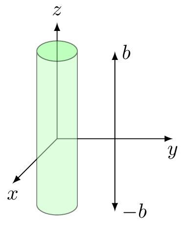
Take a very simplified cylindrical geometry radius \(a\) and length \(2b\).
In this very stylized case, there’s a trick. We can solve the problem as if there were North and South magnetic “charges” \(Q_m\) at the two faces separated by the distance \(2b\)
\[ B_z = \frac{Q_m}{4\pi} \left\{ \frac{1}{(z-b)^2} - \frac{1}{(z+b)^2} \right\} \]
Can show \[ B_z \propto \frac{1}{(z/b)^3} \]
If \(z/b = 5\) then \(B_z(5b) \approx B_z(b)/125\)
Navigable Map Metrics
Outline
- Aeromagnetic survey best practices
- Analysis of maps for navigation
Aeromagnetic survey practices for MagNav
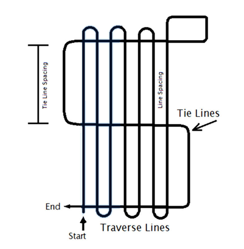
- Tolles-Lawson calibration flown before and/or after survey
- Surveys usually flown in grid pattern
- Flight lines used to model anomaly intensity
- Tie lines used for map leveling
- Local ground magnetometer reference station
- Records temporal changes of disturbance field
- (Bergeron and Nielsen 2023)
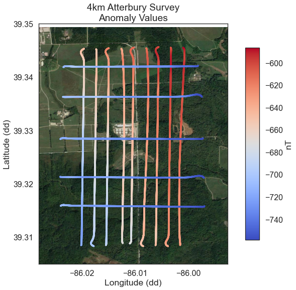
Example aeromagnetic survey flight path with dense, parallel flight lines and spare orthogonal tie lines.
Heading error and corrugation
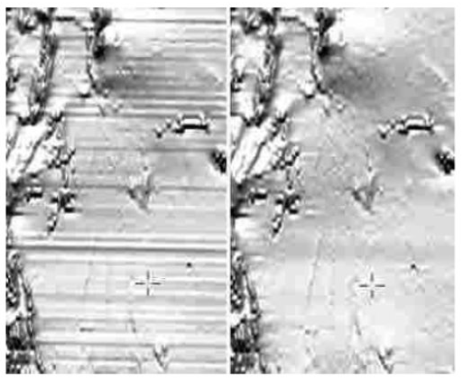
- Heading error results in corrugation
- Mitigated via map leveling
- Usually by minimizing flight/tie line intersection differences
- (Reeves 2005), (Luyendyk 1997)
- Mitigated via map leveling
Differing leveling algorithms produce different results
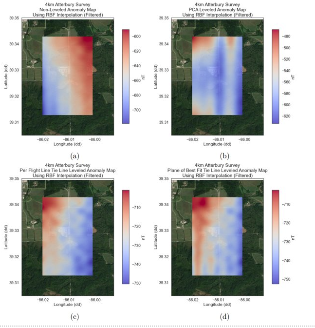
Corrugation figure of merit
- Used to determine map leveling effectiveness
- Process:
- High-pass filter in the tie-line direction
- cut-off frequency give by the survey altitude AGL
- Average in flight line direction
- Fourier transform of average
- Largest magnitude within corrugation bandwidth (\(B_c\)) selected
- \(B_c\) is the corrugation bandwidth
- \(a_{agl}\) is the survey altitude
- Invert magnitude value to obtain FOM
- \[\frac{1}{a_{agl}(1+0.05)} \le B_c \le \frac{1}{a_{agl}(1+0.05)}\]
- High-pass filter in the tie-line direction

Map comparisons
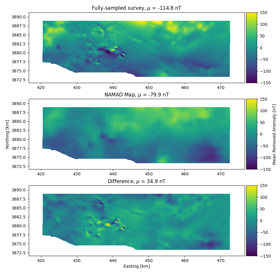
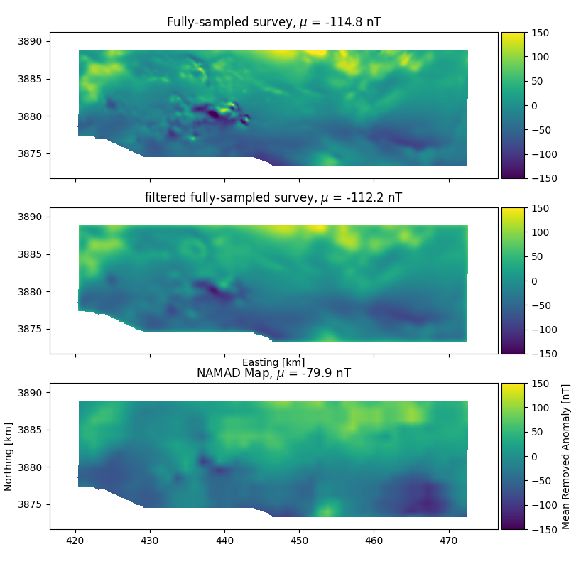
- Magnetic maps of Mojave Desert
- Both at 300 m above ground level
- NAMAD (Bankey et al. 2002)
- resolution 1.1 km
- Fully sampled
- resolution 75 m
- Obvious missing features in NAMAD
Navigation flight comparison - fully-sampled map
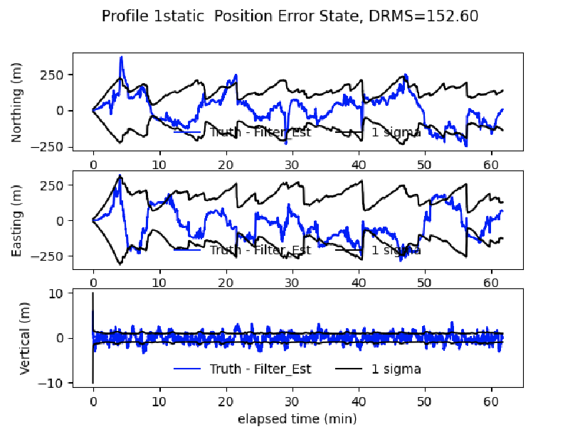
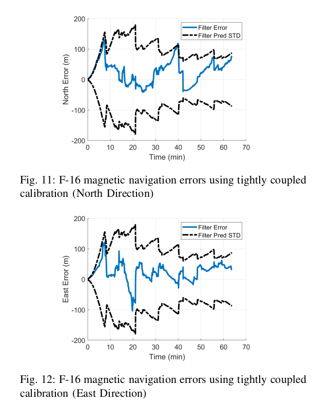
- Recent F-16 flight test demonstrated good navigation performance with a fully-sampled map
- Challenging calibration problem (\(\approx\) 5000 nT)
- Believe this to be the limiting factor to navigation performance
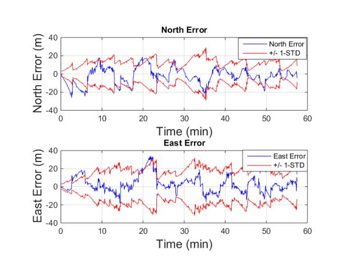
- Typical DRMS errors \(\approx\) 150 m
- (A. J. Canciani 2021), (Bonifaz 2022)
Navigation flight comparison - NAMAD map
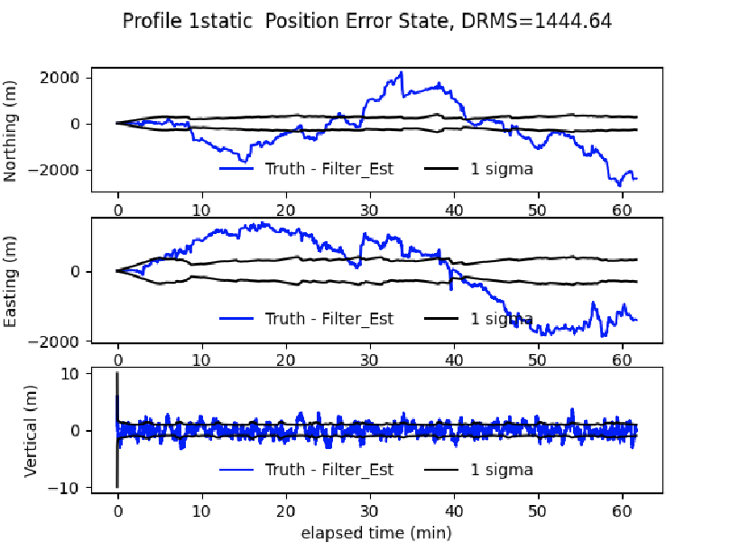
- Substitute NAMAD map in navigator
- Typical DRMS errors \(\approx\) 1500 m
- Error grows \(\approx 10\times\)
- Only difference is the map used to navigate
- NAMAD typical of existing surveys
- What features drive larger error?
- How are these features quantified?
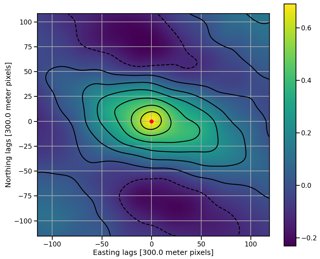
Map cross-correlation
- Filter fully-sampled map to NAMAD resolution
- 1.1 km
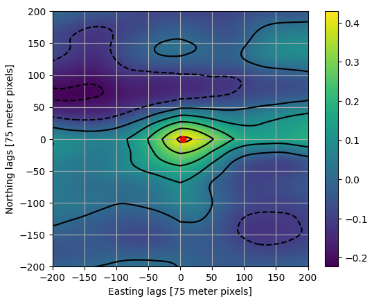
- Planar detrend both maps and perform cross-correlation
- Overall shift of 700 m between maps
Cross-correlation with fully-sampled NAMAD
- NAMAD spatial resolution becomes fully sampled at \(\approx\) 1100 m AGL
- Fully-sampled map survey flown at 2133 m AGL
- No overall shift between maps
- Registration errors masked at fully-sampled altitude

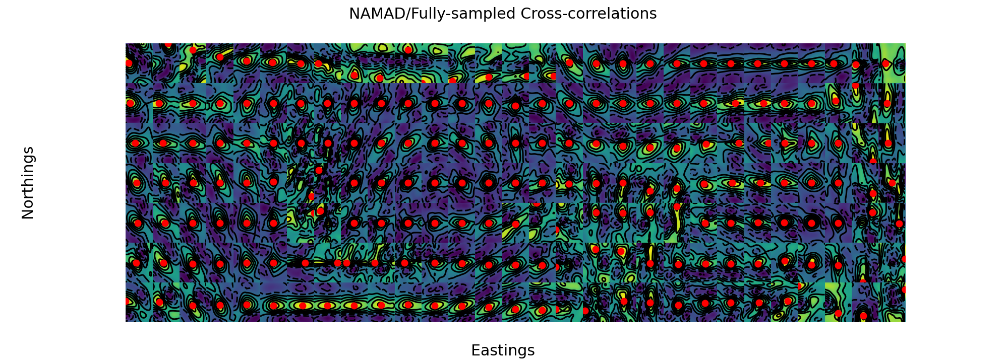
Tiled cross-correlation
- Hypothesis:
- Different regions of NAMAD need different translations to match real magnetic anomaly
- Segmented the maps into small sections
- Cross-correlate each section
- Make a map of the cross-correlation results
- Identify regions of different cross-correlation
Tiled cross-correlation results
- Identify regions of different cross-correlation properties
- specifically a shift is peak location
- Traversing from one region to another adds a shift to the navigation solution
- Breaks long-distance correlations
Underlying NAMAD data
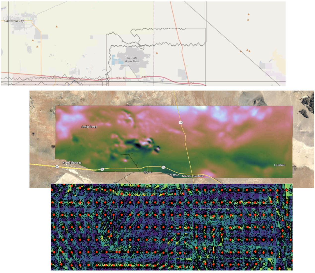
- Top Plot shows USGS survey boundaries (gray)
- Major feature in center Rio Tinto Borax Mine
- Open pit mining began 1957
- Many USGS survey in area 1954, 1955, 1978 (NURE)
- Oldest are hand-drawn digitized maps
- Survyes pre-date GPS
- Major cross-correlation peak shifts coincide with survey boundaries
Auto-correlation analysis

- NAMAD map auto-correlation differs in width and structure from fully-sampled map
- Fully-sampled map is asymmetic and longer
Auto-correlation line cuts
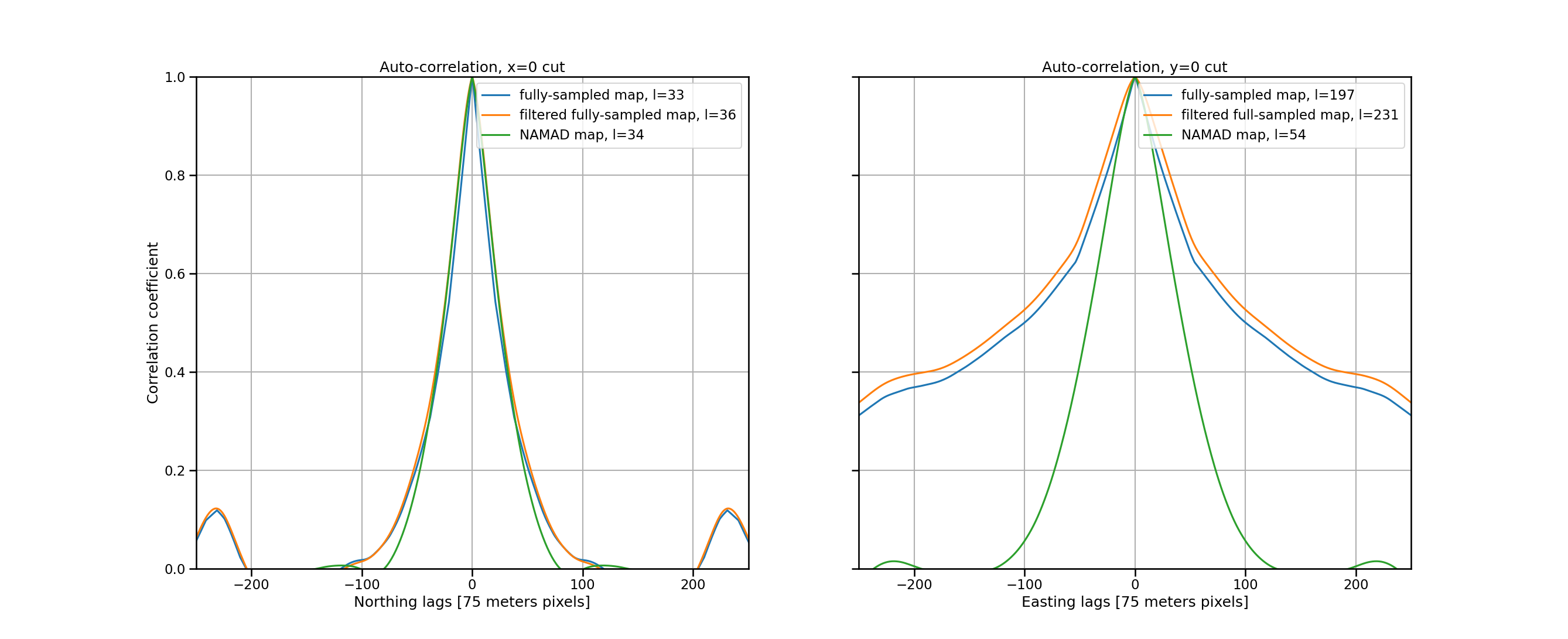
- Filtering to NAMAD spacing results in nearly same spatial correlation as unfiltered
- NAMAD map auto-correlation length
- Easting \(\approx 4 \times\) smaller than fully-sampled map
- Northing approx the same
- Geo-registration shifts in NAMAD cause loss of correlation
Power-spectral analysis
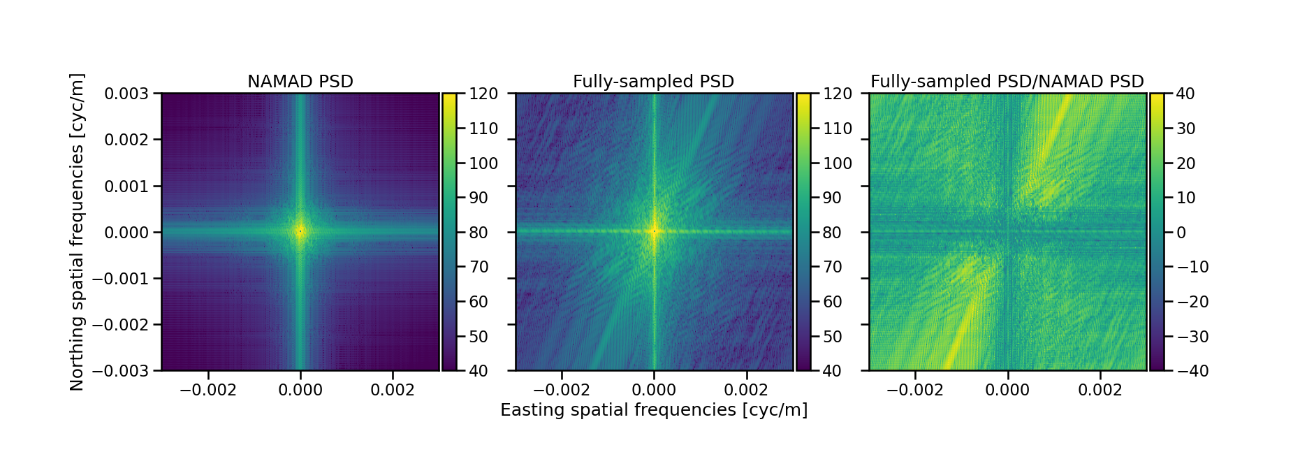
- NAMAD map confined to very narrow frequency reponse
- As much as 40 dB of energy missing at higher frequecies in NAMAD
Aircraft velocity translates spatial into temporal
- Vehicle velocity \(\vec{v}\) translates spatial magnetic anomaly into temporal anomaly
- Exponential autocorreltion length \(\ell\) in map becomes First Order Gauss-Markov process in magnetic sensor
- \(\tau = \frac{\ell}{v}\)
- Spatial frequencies \(\vec{k}\) translate into temporal frequencies \(f\)
- \(f = \vec{v} \cdot \vec{k}\)
- NAMAD auto-correlation lengths tranlsate to \(\tau\approx 30\ \text{second}\)
- F-16 Space-weather FOGM \(\tau\approx 30\ \text{second}\)
- Low-frequency map correlations accomondated by Nav filter FOGM
- High-frequency spatial content missing NAMAD
- Almost nothing left to navigate
Sensors
Magnetometer history
- Compass use documented in China 4th Century BCE (Yan 475-221 BCE)
- Gauss invented magnetometer in 1833 (Gauss 1833)
- Aschenbrenner and Goubau invented flux-gate magnetometer in 1936 (Aschenbrenner 1936)
- Vector sensor, measures one component of \(\vec{B}\)
- 3 sensors required to measure all components
- Vacquier invented airborne version of fluxgate (Vacquier 1945)
- Used gimbal to align sensor axis with total field
- Alkali vapor magnetometers (Bloom 1962) (Bell and Bloom 1957)
- Measure vector magnitude or total field \(|\vec{B}|\)
- Review article in (Tierney et al. 2019)

Vaquier towed magnetometer, National Museum of American History (Smithsonian Institution, n.d.)
History notes:
https://www.sciencenews.org/article/fluxgate-magnetometer-submarine-plate-tectonics
https://science.nasa.gov/technology/technology-highlights/rediscovering-the-lost-art-of-fluxgate-magnetometer-cores
https://geomag.nrcan.gc.ca/lab/vm/fluxgate-en.php
https://geomag.nrcan.gc.ca/lab/vm/museum-en.php
https://www.sciencenews.org/article/fluxgate-magnetometer-submarine-plate-tectonics
https://americanhistory.si.edu/collections/search/object/nmah_871581
https://faculty.epss.ucla.edu/~ctrussell/ESS265/History.html
https://wiki.seg.org/wiki/Victor_Vacquier
Scalar measurements
- Used traditionally to avoid need to measure true attitude in Earth frame
- INS not available as practical technology until 1960’s or later Smithsonian history of inertial navigation, Smithsonian Institution (n.d.)

Sensors for scalar measurements
Scalar sensors used to avoid rotation issues
Vector sensors as attitude sensors
- Could not measure your true orientation in Earth reference frame (no IMU)
- Could measure orientation around Earth field using vector sensor
- Vector could be strap-down
- Direction cosines used
- Tolles-Lawson calibration (W. E. Tolles and Lawson 1950) (W. E. Tolles 1954) (W. E. Tolles 1955) (Leliak 1961)
\[ \begin{align*} DC_x = \arccos{a} &= \frac{B_x}{\sqrt{B_x^2 + B_y^2 + B_z^2}}\\ DC_y = \arccos{b} &= \frac{B_y}{\sqrt{B_x^2 + B_y^2 + B_z^2}}\\ DC_z = \arccos{c} &= \frac{B_z}{\sqrt{B_x^2 + B_y^2 + B_z^2}} \end{align*} \]
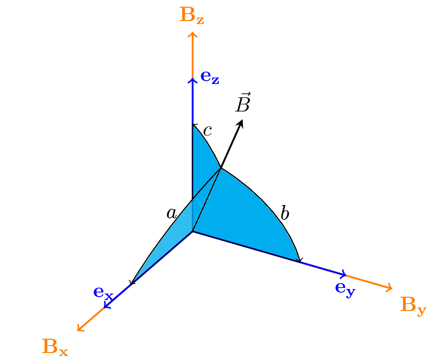
Direction cosines
- Non-linear transform that hides some potential artifacts
- For example an overall scaling of vector components divides out.
- DC derived from vector components of total field
- Computed DC will include effects of dipoles in platform reference frame
Why not just use a vector?
- Sensor requires calibration
- Mechanical - orthogonalization
- Electronic artifacts - gain and bias
- Magnetic artifacts - hard and soft bias
- Temperature dependence
Gain and bias: \[ \vec{B}_m = {\mathbf{A}_\mathrm{soft}} \vec{B}_r + \vec{b}_\mathrm{hard} \]
Hard and soft magnetic moments: \[ \vec{B}_m = {\mathbf{A}_\mathrm{soft}} \vec{B}_r + \vec{b}_\mathrm{hard} \]
Vector orthogonalization calibration techniques
- Calibration with scalar value - good review is Merayo 2000 Merayo et al. (2000)
- Fix the sensor in place and spin around
- Magnitude of \(|\vec{B}| = \mathrm{constant}\)
- Uses external reference for \(|\vec{B}|\)
- Orthogonalization correction
- \(\vec{B}_m = A \left[\vec{B}_r + \vec{b} \right]\)
- \(A\) is a triangular matrix
- \(b\) is a bias vector
Hard and soft iron bias calibration
- Commonly advertised technique for inexpensive magnetometers
- Hard - permanent moments
- Soft - induced moments
- Typically a rotational test \(|\vec{B}| = \mathrm{constant}\)
- \(\vec{B}_m = A \left[\vec{B}_r + \vec{b} \right]\)
- \(A\) is symmetric matrix
- \(b\) is the permanent moment bias
Vector calibration example
- Before calibration, the vector magnetometer lies on a shifted ellipse.
- After calibration, the vector magnetomter values will lie on the surface of a sphere.
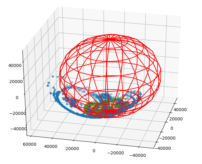
- blue - before calibration
- green -after calibration
- red - fixed magnitude sphere
Temperature dependence
Newton’s law of cooling \[T(t) = T_s +(T_0 - T_s)\exp(-kt)\] which is the solution to \[\frac{dT}{dt} = -k(T_0 - T_s)\] if \(H \propto T\) then we can write by analogy \[H(t) = H_f + (H_0 - H_f)\exp(-kt)\]
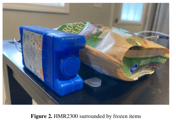
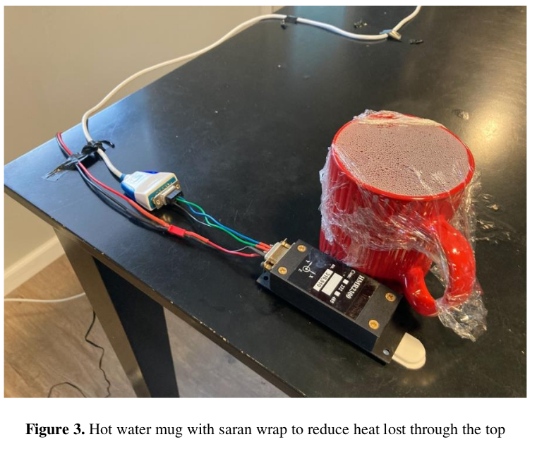
Temperature compensation
Newton’s law of cooling \[T(t) = T_s +(T_0 - T_s)\exp(-kt)\] which is the solution to \[\frac{dT}{dt} = -k(T_0 - T_s)\] if \(H \propto T\) then we can write by analogy \[H(t) = H_f + (H_0 - H_f)\exp(-kt)\]
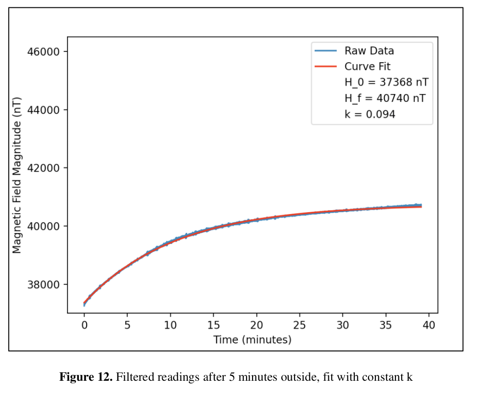
Scalar sensors
Scalar sensor has advantage that it’s output independent of magnetic field orientation.
Generally we refer to Atomic vapor sensors.
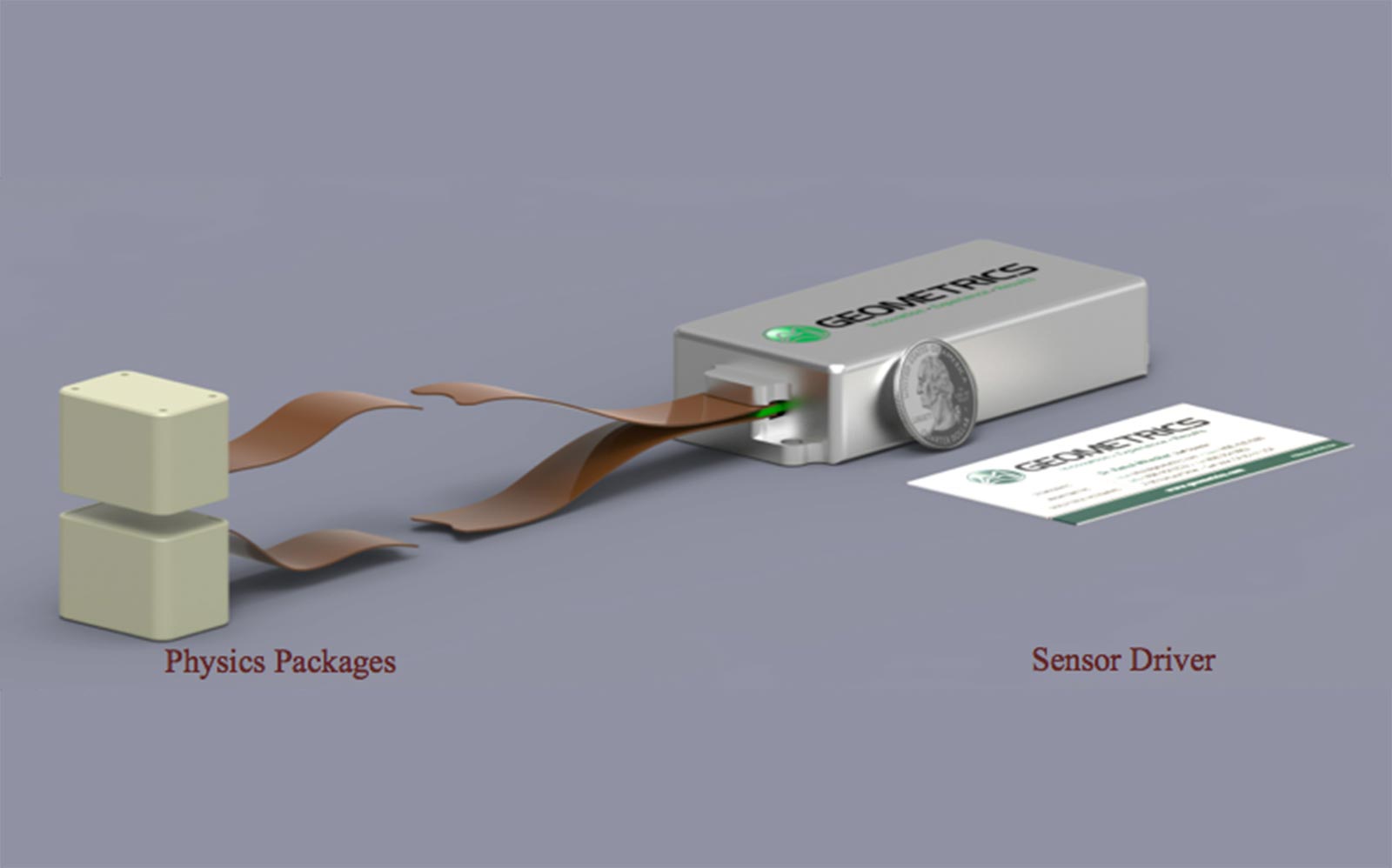
Geometrics MFAM (MFAM Module Specifications, Laser Pumped Cesium Magnetometer 2020)
Interpretation of scalar value in geomagnetic context
\[ \begin{align*} |\vec{B}_\mathrm{total}| &= |\vec{B}_\mathrm{Earth} + \vec{B}_\mathrm{anomaly}|\\ &= \sqrt{ |B_\mathrm{Earth}|^2 + |B_\mathrm{anomaly}|^2 + 2 |B_\mathrm{Earth}||B_\mathrm{anomaly}|\cos\theta}\\ |B_\mathrm{total}| &= |B_\mathrm{Earth}| \sqrt{ 1 + \frac{|B_\mathrm{anomaly}|^2}{|B_\mathrm{Earth}|^2} + 2\frac{|B_\mathrm{anomaly}|}{|B_\mathrm{Earth}|}\cos\theta } \\ &\approx |B_\mathrm{Earth}| + |B_\mathrm{anomaly}|\cos\theta + \cdots \end{align*} \]
\(|B_\mathrm{anomaly}|\) is the projection of \(\vec{B}_\mathrm{anomaly}\) onto \(\vec{B}_\mathrm{Earth}\)


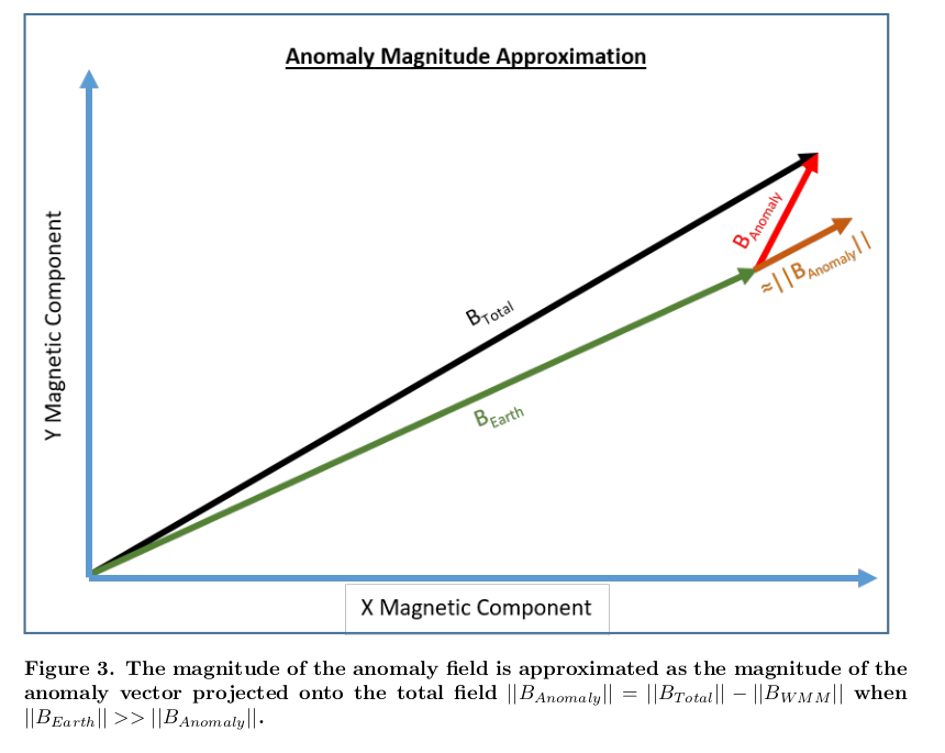
Atomic sensors - Larmor precession
Atomic vapor sensors operate on the principle of Larmor precession
These are gases that have an unpaired electron that has a specific magnetic moment.
Cesium \(\gamma = 3.5\ \text{nT/Hz}\)
In Earth field of \(50000\ \text{nT} \rightarrow 175 \text{kHz}\)
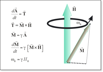
- \(\vec{A}\) is angular momentum
- \(\vec{T}\) is torque
- \(\vec{M}\) is magnetic moment
- \(\vec{H}\) is magnetic field
- \(\gamma\) is gyromagnetic ratio
Atomic sensor operation
Inside the sensor head is the Ce gas. Without doing anything the atoms in the gas have a random orientation.
A pump laser with a specific polarization orients the Ce spins and excites them to a specific state.
A probe laser reads out the precesion rate and the magnetic field is inferred.
The probe laser is polarized so that it is absorbed by the Ce gas when the spin aligns with the beam polarization.
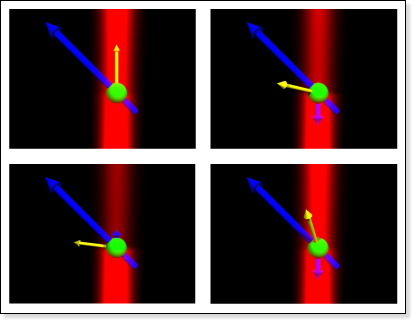
- Geometrics
- Red - probe laser beam
- Blue - magnetic field
- Yellow - magnetic moment
Atomic sensor issues
- How to interpret signal in geomagnetic context
- Primary sensor issues
- Deadzones
- Heading errors
Deadzone
Related to the pump laser optical axis.
Pump laser is circular polarized and transfers angular momentum to the atoms so that they spin align to the optical axis \((\vec{M}\parallel\text{optical\ axis})\)
Torque \(\vec{T}\) on \(\vec{M}\) from \(\vec{H}\) is: \[ \vec{T} = \vec{M} \times \vec{H} \] If \(\vec{M} \parallel \vec{H}\), then \(\vec{T} = \vec{M} \times \vec{H} = 0\)
No torque \(\rightarrow\) no precession and no signal to monitor.
Details of laser-gas interaction define deadzone size.
Deadzone avoidance
- Orient optical axis based on knowledge of external field
- OK if external field does not move - not practical for vehicles
- Use multiple sensors
- arrange so that one is always out of deadzone, how many do you need?
- travel from Northern to Southern hemisphere
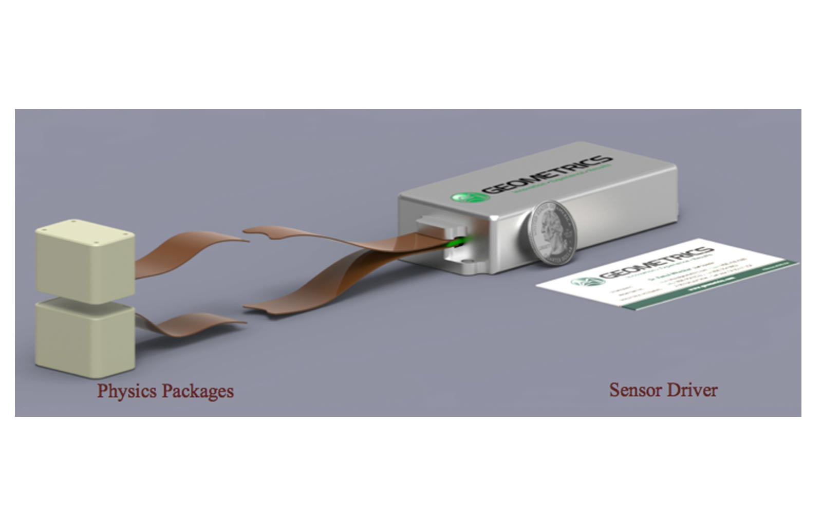
Geometrics MFAM (MFAM Module Specifications, Laser Pumped Cesium Magnetometer 2020)
Heading error
Heading error is due to small amounts of magnetization near the sensor and leads to an orientation dependent bias.
\(\cos\theta\) is the angle between \(\vec{B}_\mathrm{external}\) and \(\vec{B}_\mathrm{sensor}\).
\[ \begin{align*} |\vec{B}_\mathrm{measure}| &= |\vec{B}_\mathrm{external} + \vec{B}_\mathrm{sensor}|\\ &= \sqrt{ |B_\mathrm{external}|^2 + |B_\mathrm{sensor}|^2 + 2 |B_\mathrm{external}||B_\mathrm{sensor}|\cos\theta}\\ |B_\mathrm{measure}| &= |B_\mathrm{external}| \sqrt{ 1 + \frac{|B_\mathrm{sensor}|^2}{|B_\mathrm{external}|^2} + 2\frac{|B_\mathrm{sensor}|}{|B_\mathrm{external}|}\cos\theta} \\ &\approx |B_\mathrm{external}| + |B_\mathrm{sensor}|\cos\theta + \cdots \end{align*} \]
Multiple vector sensors
The full magnetic vector gradient has 9 components \[ \nabla \vec{B} = \begin{bmatrix} \frac{\partial}{\partial x}\\ \frac{\partial}{\partial y}\\ \frac{\partial}{\partial z} \end{bmatrix} \begin{bmatrix} B_x & B_y & B_z \end{bmatrix} = \begin{bmatrix} \frac{\partial B_x}{\partial x} & \frac{\partial B_x}{\partial y} & \frac{\partial B_x}{\partial z} \\ \frac{\partial B_y}{\partial x} & \frac{\partial B_y}{\partial y} & \frac{\partial B_y}{\partial z} \\ \frac{\partial B_z}{\partial x} & \frac{\partial B_z}{\partial y} & \frac{\partial B_z}{\partial z} \end{bmatrix} \]
Maxwell’s equations provide constraints, trace must be zero \[ \nabla \cdot \vec{B} = 0 \] In free space \[ \nabla \times \vec{B} = 0 \] Which means that \(\nabla \vec{B}\) must be symmetric
Only 5 independent elements (Bracken and Brown 2006).
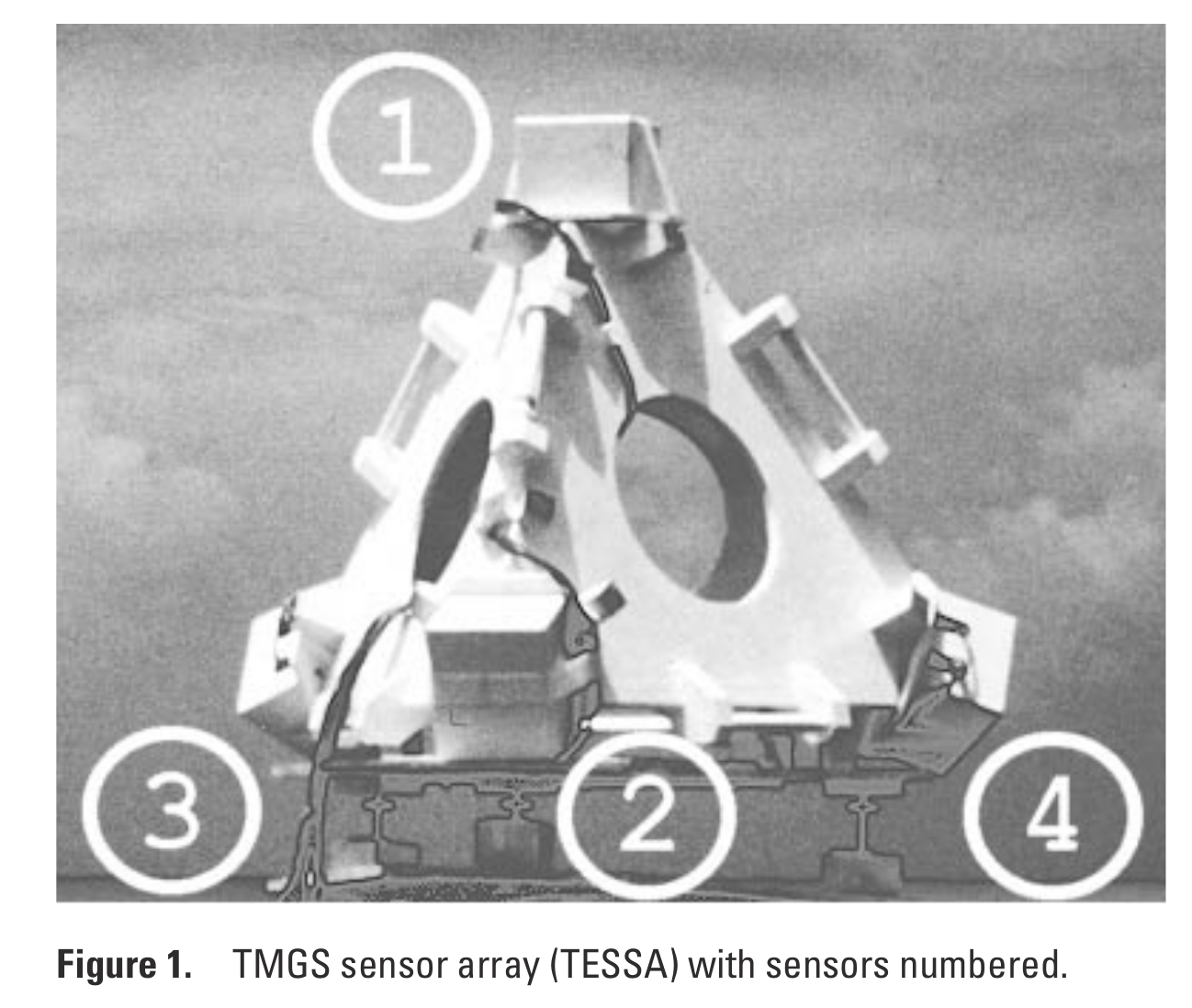
Vector Gradiometer aka Tensiometer
Because of the contraints, a vector gradiometer can be made with \(\ge 4\) vector sensors in a cross (plane) or in a tetrahedron or similar shape.
Magnetic field gradients
\[ \vec{B}_\mathrm{dipole} = \frac{\mu_0 }{4\pi} { \frac{1}{r^3} }\left[ 3 (\vec{m}\cdot \hat{r})\hat{r} - \vec{m} \right] \propto \frac{1}{r^3} \]
\[ | (\nabla \vec{B}_\mathrm{dipole})_{ij}| \propto \frac{1}{r^4} \]
Differencing two measurements will will remove a constant and leave behind what’s different.
The closer a dipole, the steeper the gradient.
Gradient measurements will be dominated by local dipoles.
Compensation and Calibration
Traditional Tolles-Lawson calibration
An airplane is a big magnet that flies

\(|\vec{B}_\text{sensor}| = |\vec{B}_{\oplus}+ \vec{B}_\text{anomaly}+ \vec{B}_\text{disturbance}+ \vec{B}_\class{fa fa-plane}{}|\)
An airplane is a big magnet that flies
\(|\vec{B}_\text{sensor}| = |\vec{B}_{\oplus}+ \vec{B}_\text{anomaly}+ \vec{B}_\text{disturbance}+ \vec{B}_\class{fa fa-plane}{}|\)
\(|\vec{B}_\text{ext}| = |\vec{B}_{\oplus}+ \vec{B}_\text{anomaly} + \vec{B}_\text{disturbance}|\)
\(|\vec{B}_\text{sensor}| = |\vec{B}_\text{ext}+ \vec{B}_\class{fa fa-plane}{}|\)
assume \(|\vec{B}_\class{fa fa-plane}{}|/|\vec{B}_\text{ext}|\ll 1\)
\(|\vec{B}| \approx |\vec{B}_\text{ext}| + \frac{1}{2}\vec{B}_\class{fa fa-plane}{}\cdot\vec{B}_\text{ext}\)
need a model for \(\vec{B}_\class{fa fa-plane}{}\)

Tolles-Lawson
- Calibration technique developed in WW2 for submarine hunting
- Declassified in 1950’s and patented
- Standard calibration technique used for aero-magnetic surveys
- Developed by (Leliak 1961)
\[ \begin{align*} |B_\text{sensor}| &= |\vec{B}_\text{ext}+ \vec{B}_\class{fa fa-plane}{}|\\ &= \sqrt{ |B_\text{ext}|^2 + |B_\class{fa fa-plane}{}|^2 + 2 |B_\text{ext}||B_\class{fa fa-plane}{}|\cos\theta}\\ |B_\text{sensor}| &= |B_\text{ext}| \sqrt{ 1 + \frac{|B_\class{fa fa-plane}{}|^2}{|B_\text{ext}|^2} + 2\frac{|B_\class{fa fa-plane}{}|}{|B_\text{ext}|}\cos\theta} \end{align*} \]
Tolles-Lawson
- Calibration technique developed in WW2 for submarine hunting
- Declassified in 1950’s and patented
- Standard calibration technique used for aero-magnetic surveys
- Developed by (Leliak 1961)

\[ \begin{align*} |B_\text{sensor}| &= |\vec{B}_\text{ext}+ \vec{B}_\class{fa fa-plane}{}|\\ &= \sqrt{ |B_\text{ext}|^2 + |B_\class{fa fa-plane}{}|^2 + 2 |B_\text{ext}||B_\class{fa fa-plane}{}|\cos\theta}\\ |B_\text{sensor}| &= |B_\text{ext}| \sqrt{1 + 2\frac{|B_\class{fa fa-plane}{}|}{|B_\text{ext}|}\cos\theta} \end{align*} \]
Tolles-Lawson Path to Calibration 1/2
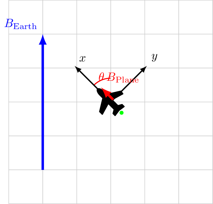
\[
\begin{align*}
|B_\text{Sensor}| &= |\vec{B}_\text{ext}+ \vec{B}_\class{fa fa-plane}{}|\\
&= \sqrt{ |B_\text{ext}|^2 + |B_\class{fa fa-plane}{}|^2 + 2 |B_\text{ext}||B_\class{fa fa-plane}{}|\cos\theta}\\
|B_\text{Sensor}| &= |B_\text{ext}| \sqrt{ 1 + 2\frac{|B_\class{fa fa-plane}{}|}{|B_\text{ext}|}\cos\theta}\\
&\approx |B_\text{ext}| + |B_\class{fa fa-plane}{}|\cos\theta + \cdots
\end{align*}
\]
Path to Calibration
Measure \(\cos\theta\)
Solve \(|B_\text{sensor}| = |B_\text{ext}| + |B_\class{fa fa-plane}{}|\cos\theta\)
Assuming \(|B_\text{ext}|\) is known or constant
Tolles-Lawson Path to Calibration 2/2

Path to Calibration
Measure \(\cos\theta\)
Solve \(|B_\text{sensor}| = |B_\text{ext}| + |B_\class{fa fa-plane}{}|\cos\theta\)
Assuming \(|B_\text{ext}|\) is known or constant
How to measure \(\cos\theta\)?
Use a vector magnetometer
Rotate aircraft in \(\vec{B}_\text{ext}\)
Direction cosines
- The direction cosines are computed in the vector magnetometer reference frame
- The magnetometer is fixed to aircraft body reference frame \[ \begin{aligned} \cos X = & \frac{B_x}{\sqrt{B_x^2 + B_y^2 + B_z^2}}\\ \cos Y = & \frac{B_y}{\sqrt{B_x^2 + B_y^2 + B_z^2}}\\ \cos Z = & \frac{B_z}{\sqrt{B_x^2 + B_y^2 + B_z^2}} \end{aligned} \]
Calibration 1/4
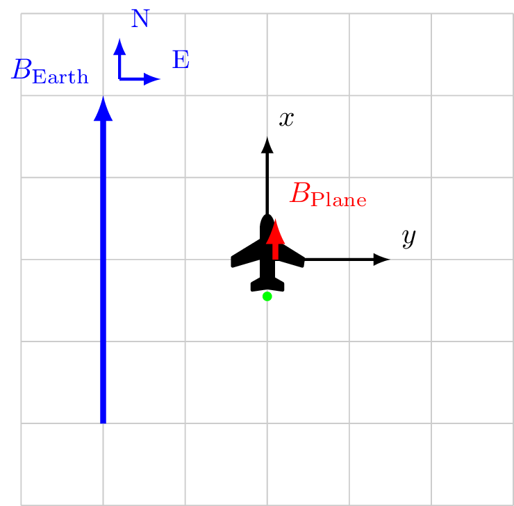
Coordinate system fixed to aircraft
\[\vec{B}_\text{Sensor} = \vec{B}_\text{ext}+ \vec{B}_\class{fa fa-plane}{}\]
\[
\begin{alignat*}{3}
\vec{B}_\text{ext}&= 4.0 \hat{x} && + 0.0 \hat{y} \\
\vec{B}_\class{fa fa-plane}{}&= 0.5 \hat{x} && +0.0 \hat{y} \\
\vec{B}_\text{Sensor} &= 4.5 \hat{x} && + 0.0 \hat{y} \\
|B_\text{Sensor}| &= 4.5 && \\
\cos X &= \frac{4.5}{4.5} && = 1\\
\cos Y &= \frac{0.0}{4.5} && = 0\\
\end{alignat*}
\]
Calibration 2/4
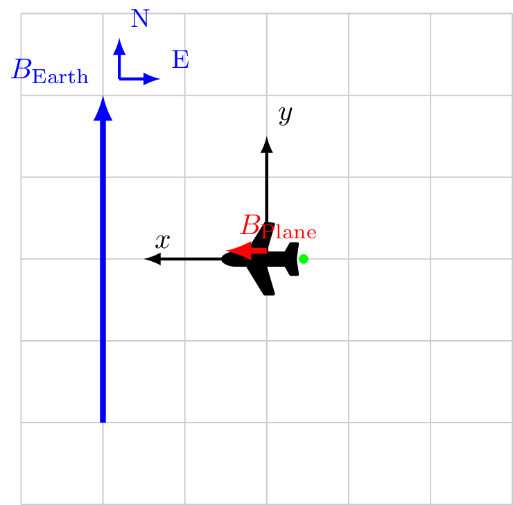
Coordinate system fixed to aircraft
\[\vec{B}_\text{Sensor} = \vec{B}_\text{ext}+ \vec{B}_\class{fa fa-plane}{}\]
\[
\begin{alignat*}{3}
\vec{B}_\text{ext}&= 0.0 \hat{x} && + 4.0 \hat{y} \\
\vec{B}_\class{fa fa-plane}{}&= 0.5 \hat{x} && + 0.0 \hat{y} \\
\vec{B}_\text{Sensor} &= 0.5 \hat{x} && + 4.0 \hat{y} \\
|B_\text{Sensor}| &= 4.007 && \\
\cos X &= \frac{0.5}{4.007} && \ne 0 \rightarrow 82.8^\circ\\
\cos Y &= \frac{4.0}{4.007} && \approx 1\\
\end{alignat*}
\]
Calibration 3/4
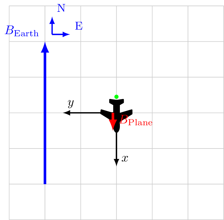
Coordinate system fixed to aircraft
\[\vec{B}_\text{Sensor} = \vec{B}_\text{ext}+ \vec{B}_\class{fa fa-plane}{}\]
\[
\begin{alignat*}{3}
\vec{B}_\text{ext}&= -4.0 \hat{x} && + 0.0 \hat{y} \\
\vec{B}_\class{fa fa-plane}{}&= 0.5 \hat{x} && + 0.0 \hat{y} \\
\vec{B}_\text{Sensor} &= -3.5 \hat{x} && + 0.0 \hat{y} \\
|B_\text{Sensor}| &= 3.5 && \\
\cos X &= \frac{-3.5}{3.5} && = -1\\
\cos Y &= \frac{0}{3.5} && = 0\\
\end{alignat*}
\]
Calibration 4/4
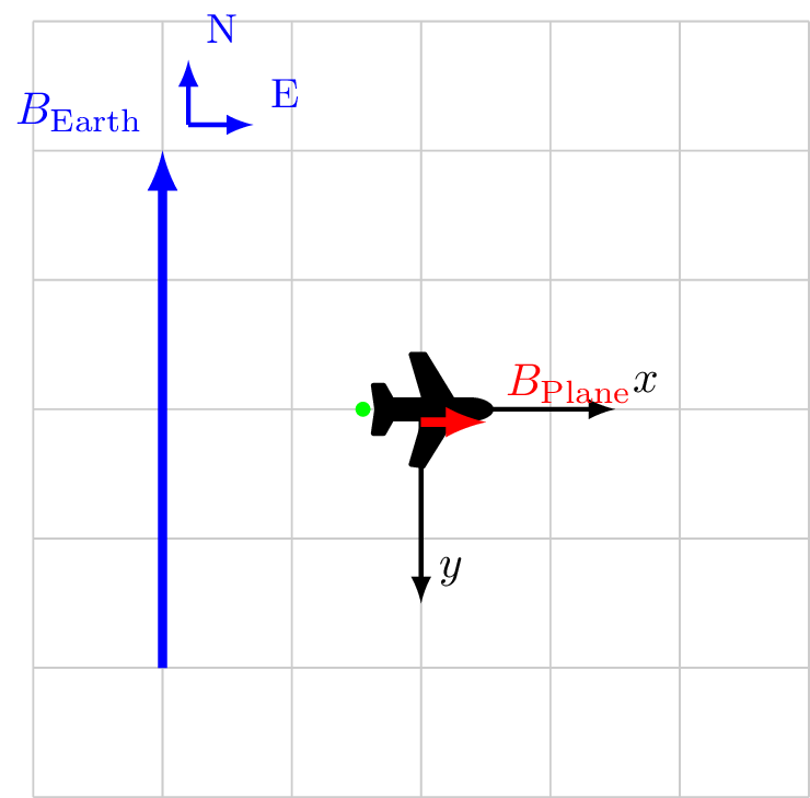
Coordinate system fixed to aircraft
\[\vec{B}_\text{Sensor} = \vec{B}_\text{ext}+ \vec{B}_\class{fa fa-plane}{}\]
\[
\begin{alignat*}{3}
\vec{B}_\text{ext}&= 0.0 \hat{x} && + -4.0 \hat{y} \\
\vec{B}_\class{fa fa-plane}{}&= 0.5 \hat{x} && + 0.0 \hat{y} \\
\vec{B}_\text{Sensor} &= 0.5 \hat{x} && + -4.0 \hat{y} \\
|B_\text{Sensor}| &= 4.007 &&\\
\cos X &= \frac{0.5}{4.007} && \ne 0\\
\cos Y &= \frac{-4.0}{4.007} && \approx -1\\
\end{alignat*}
\]
Standard calibration model - Tolles-Lawson
\[|\vec{B}_\text{sensor}| = |\vec{B}_\text{ext}+ \vec{B}_\class{fa fa-plane}{}|\]
\[ \begin{array}{ l B c B c B c } \vec{B}_\class{fa fa-plane}{}& = & \vec{B}_\text{Permanent} & + & \vec{B}_\text{Induced} & + & \vec{B}_\text{Eddy}\\ & = & \vec{P}_\text{constant} {} & + &{} M_{3\times3} \vec{B}_\text{ext}{} & + & {} S_{3\times3} \frac{\partial}{\partial t} \vec{B}_\text{ext} \end{array} \]
\(M_{3\times3}\) is symmetric \(\rightarrow\) 6 independent elements
Total of 18 elements
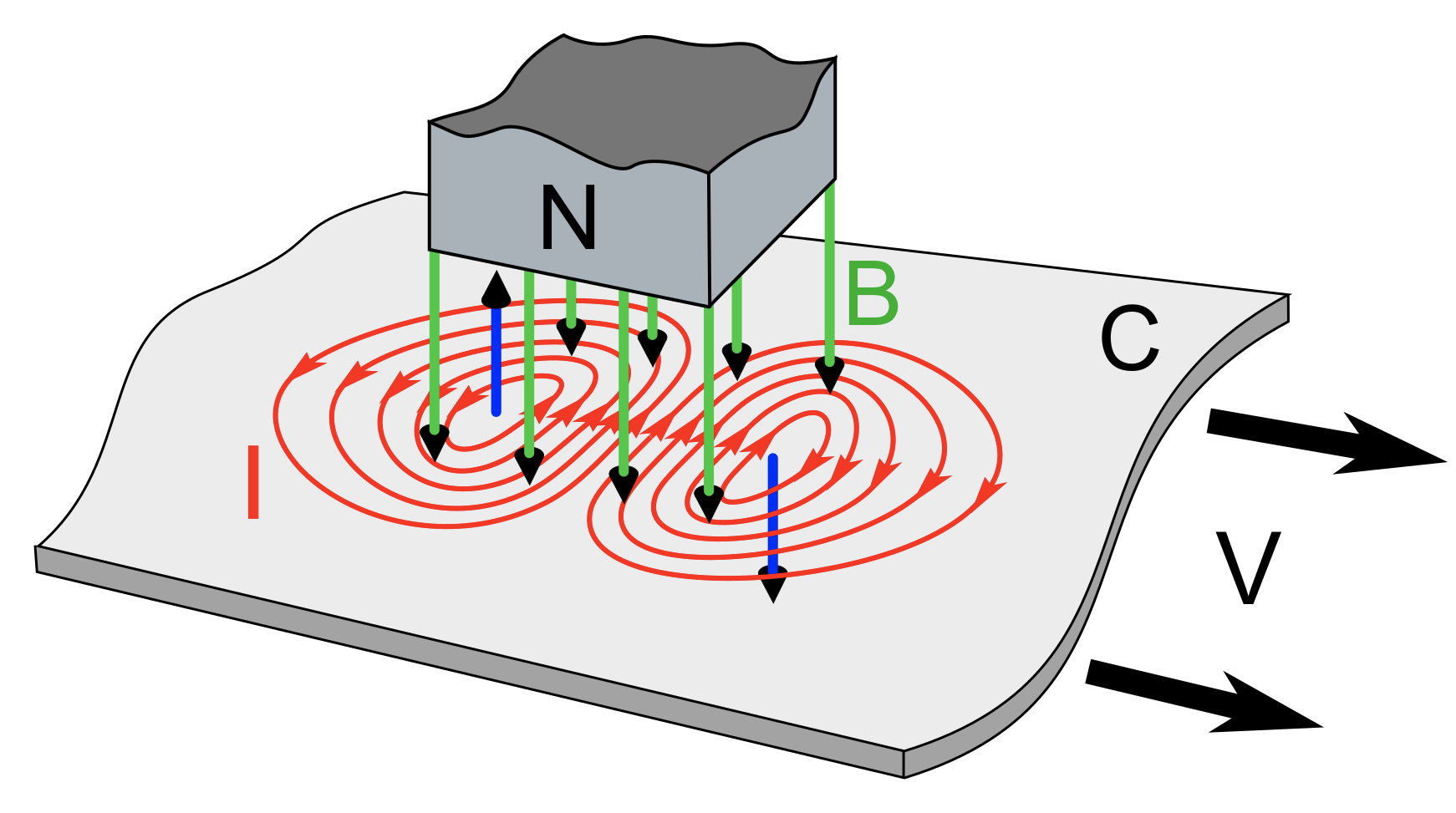
Use the same direction cosines, now with \(B_z\)
The direction cosines are computed from the vector magnetometer
\[ \begin{aligned} \cos X = & \frac{B_x}{\sqrt{B_x^2 + B_y^2 + B_z^2}}\\ \cos Y = & \frac{B_y}{\sqrt{B_x^2 + B_y^2 + B_z^2}}\\ \cos Z = & \frac{B_z}{\sqrt{B_x^2 + B_y^2 + B_z^2}} \end{aligned} \]
Tolles-Lawson full implementation
\[
\begin{aligned}
B_\class{fa fa-plane}{}& = & & { c_1 \cos X + c_2 \cos Y + c_3 \cos Z }+ \\
& & B_\text{ext}& {[ c_4 \cos^2 X + c_5 \cos X \cos Y + c_6 \cos X \cos Z +} \\
& & & { c_7 \cos^2 Y + c_8 \cos Y \cos Z + c_9 \cos^2 Z ] + } \\
& & B_\text{ext}& { [ c_{10} \cos X \cos' X + c_{11} \cos X \cos' Y + c_{12} \cos X \cos' Z }+ \\
& & & { c_{13} \cos Y \cos' X + c_{14} \cos Y \cos' Y + c_{15} \cos Y \cos' Z +} \\
& & & { c_{16} \cos Z \cos' X + c_{17} \cos Z \cos' Y + c_{18} \cos Z \cos' Z ] }
\end{aligned}
\]
- We need a method to solve for \(c_1 \ldots c_{18}\) - Should provide visibility over anticipated range of aircraft motion
Calibration manuevers - Tolles-Lawson
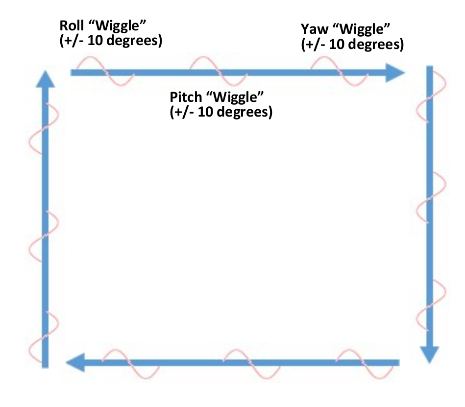
Fly the aircraft in a series of Roll, Pitch, Yaw maneuvers
High-altitude
Altitude of a known map
Maneuver angle should depend upon the expected aircraft dynamics
- Barrel Rolls?
Typically at each cardinal heading
- 3 rolls \(\pm 10^\circ\) at 1 Hz
- 3 pitches \(\pm 10^\circ\) at 1 Hz
- 3 yaws \(\pm 10^\circ\) at 1 Hz
(W. E. Tolles and Lawson 1950), (W. E. Tolles 1954), (W. E. Tolles 1955), (Gnadt, Wollaber, and Nielsen 2022)
Construct Tolles-Lawson \(A\) matrix
\[ A = \begin{bmatrix} \cos X_1 & \cdots & \cos X_N\\ \cos Y_1 & \cdots & \cos Y_N \\ \cos Z_1 & \cdots & \cos Z_N\\ B_\text{ext}\cos^2 X_1 & \cdots & B_\text{ext}\cos^2 X_N\\ B_\text{ext}\cos X_1 \cos Y_1 & \cdots & B_\text{ext}\cos X_N \cos Y_N\\ B_\text{ext}\cos X_1 \cos Z_1 & \cdots & B_\text{ext}\cos X_N \cos Z_N \\ B_\text{ext}\cos^2 Y_1 & \cdots & B_\text{ext}\cos^2 Y_N \\ B_\text{ext}\cos Y_1 \cos Z_1 & \cdots & B_\text{ext}\cos Y_N \cos Z_N\\ B_\text{ext}\cos^2 Z_1 & \cdots & B_\text{ext}\cos^2 Z_N\\ B_\text{ext}\cos X_1 \cos' X_1 & \cdots & B_\text{ext}\cos X_N \cos' X_N \\ B_\text{ext}\cos X_1 \cos' Y_1 & \cdots & B_\text{ext}\cos X_N \cos' Y_N\\ B_\text{ext}\cos X_1 \cos' Z_1 & \cdots & B_\text{ext}\cos X_N \cos' Z_N\\ B_\text{ext}\cos Y_1 \cos' X_1 & \cdots & B_\text{ext}\cos Y_N \cos' X_N\\ \vdots & & \vdots \\ B_\text{ext}\cos Z_1 \cos' Z_1 & \cdots & B_\text{ext}\cos Z_N \cos' Z_N \\ \end{bmatrix} \]
\(H_e\) is the magnitude of the external field. We assume that \[
B_\text{ext}= \sqrt{B_x^2 + B_y^2 + B_z^2}
\]
Equivalently that the vector mags only see external field. The anomaly signal is below the noise floor.
Solve for the \(c_i\) coefficients
Map-less calibration
Perform maneuvers at fixed frequency \(f\)
Band-pass filter columns of \(A\), \(B_\text{scalar}\) \[
\begin{aligned}
A_f & = BPF(A)\\
B_{\text{scalar},f} & = BPF(B_{\text{scalar}})
\end{aligned}
\]
Solve for \(c\)
\[
A_f \cdot c = B_{\text{scalar},f}
\]
Map-based calibration
Perform maneuvers over known-good map
Solve for \(c\)
\[
A \cdot c = B_{\text{scalar}} - B_{{\oplus}} - B_{\text{anomaly}}
\]
Multi-colinearity in solution
- There is multi-colinearity in the A-matrix via two constraints
- \(\cos^2 X + \cos^2 Y + cos^2 Z = 1\)
- \(\cos' X \cos X + \cos' Y \cos Y + \cos'Z \cos Z = 0\)
- Solving \(A^T c^T = B_\class{fa fa-plane}{}\) is overdetermined
- The standard solution is ordinary least squares \[ \begin{aligned} Ac & = B_\class{fa fa-plane}{}\\ A^T A c & = A^T B_\class{fa fa-plane}{}\\ c & = (A^T A)^{-1} A^T B_\class{fa fa-plane}{} \end{aligned} \]
- This is effectively what numpy’s
np.linalg.lstsqperforms. - Often this works just fine
Ridge regression
- If there is multi-colinearity, Ridge regression is one technique that can be used
- Solve inteads: \[c = \left( (A^T A+ kI)^{-1} A^T \right) B_\class{fa fa-plane}{}\]
- \(k\) is called the Ridge parameter since it’s along the diagonal and it should be small
- \(k=0\) is standard linear regression
- Otherwise must determine hyper-parameter \(k\)
- Python package
scikit-learnprovidesRidgeandRidgeCVroutines to do this
Ridge regression
- Ridge regression results generally less dependent upon small changes to the data
- More robust to noisy data
- Goal of ridge regression is not to find the smallest error
- Goal is to find a solution that is less sensitive to small variations in input data
- May produce a biased result
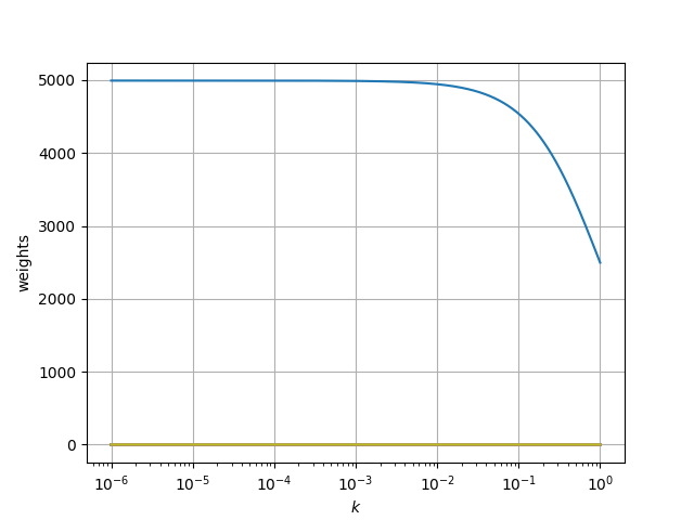
Finding ridge regression hyper-parameter \(k\)
- \(k \rightarrow \infty\) leads to \(c=0\)
- \(k = 0\) leads to regular least squares
- Examine “Ridge Trace” Plot
- Identify where the \(c\) stabilize
Finding ridge regression hyper-parameter \(k\)
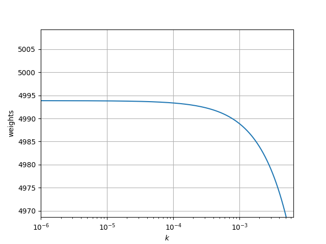
- \(k \rightarrow \infty\) leads to \(c=0\)
- \(k = 0\) leads to regular least squares
- Examine “Ridge Trace” Plot
- Identify where the \(c\) stabilize
- In this case \(k\approx 1\times10^{-4}\)
Finding ridge regression hyper-parameter \(k\)
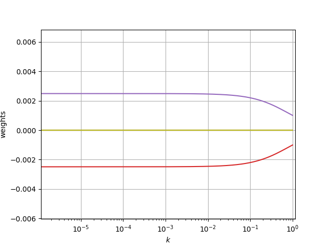
- \(k \rightarrow \infty\) leads to \(c=0\)
- \(k = 0\) leads to regular least squares
- Examine “Ridge Trace” Plot
- Identify where the \(c\) stabilize
- In this case \(k\approx 1\times10^{-4}\)
Apply \(c\) to in-flight data for comparison
In-flight
Compute \(A_k\) for each time-step
Apply \(c\)
\[
B_\class{fa fa-plane}{}= A \cdot c
\]
\[
B_\text{anomaly}= B_\text{sensor}- B_{\oplus}- B_\class{fa fa-plane}{}
\]
Navigation Algorithrms
Magnetic Navigator
- Uses an Inertial Navigation System (INS)
- barometer used for altitude stabilization
- Magnetic Navigation is a map-matching process
- sequential estimation
- single measurement value compared to map
- Navigator
- provides error correction to the drifting INS solution
- Kalman filter variant
- Extended Kalman filter
- appropriate state vector - Pinson15
- Cramer-Rao Lower bound
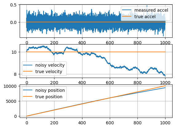
Inertial Navigation
- Inertial Measurement Unit (IMU)
- measures accelerations \(\vec{f}\)
- measures rotation rates \(\dot{\vec{\theta}}\)
- To get position from accleration, you have to integrate twice
- continuously adds noise to your position estimate
- Drifting position estimate needs to be corrected
- MagNav!
Required data sources
- Inertial Navigation System (INS)
- Angle rates, \(\Delta\theta\)
- Accelerations/specific forces, \(\Delta\vec{v}\)
- Barometer
- Precise but not accurate
- Stablize the altitude
- Magnetometers
- Scalar - primary sensor
- Vector - for compensation
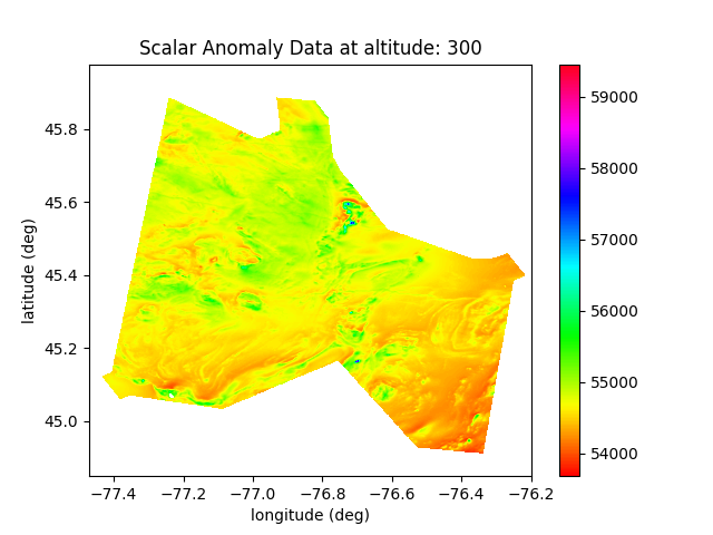
- Magnetic Map
- Core field model e.g. WMM or IGRF
- Magnetic anomaly map

Navigator overview - Extended Kalman Filter
State vector
\[ \vec{x}= \begin{bmatrix} \smash[b]{\underbrace{\begin{matrix} \delta \vec{p} & \delta \vec{v} & \delta \vec{\epsilon} & \vec{b}_a & \vec{b}_g\end{matrix}}_{\text{Pinson 15}}} & \smash[b]{\underbrace{\begin{matrix}\delta h_a & \delta a\end{matrix}}_{\text{Baro}}} & S_\text{fogm} & S_\text{bias} \end{bmatrix} \]
Measurement processor
\[ z = h(\vec{x}) + v \] \[ h(\vec{x}) = |B_\mathrm{a}| + |B_\text{earth}| + {\color{gray}|B_\text{Plane}}| + S_\text{fogm} + S_\text{bias} \]
Where
- \(|B_\mathrm{a}|\) comes from map interpolation
- \(|B_\text{earth}|\) World Magnetic Model
- \(|B_\text{Plane}|\) aircraft disturbance field - not included here with SGL calibration
- \(S_\text{fogm}\) scalar state estimates of space-weather
- \(S_\text{bias}\) offset bias between map and measurement
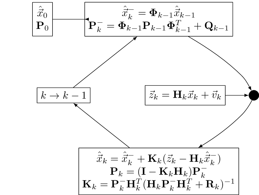
Kalman filter review
Discrete time dynamics at time index \(k+1\) the state vector \(\vec{x}_{k+1}\) is \[ \vec{x}_{k+1} = {\Phi}_k \vec{x}_k + {B}_k \vec{u}_k + \vec{w}_k \]
- \(\Phi_k\) is the state transition matrix
- \(B_k\) is the input or control matrix
- we are not supplying control, so \(B=0\)
- we are not supplying control, so \(B=0\)
- \(\vec{w}\sim \mathcal{N}(0,{Q})\) is Gaussian white noise process with covariance matrix \({Q}\)
A measurement \(\vec{z}\) is \[ \vec{z}_k = {H}_k \vec{x}_k + \vec{v}_k \]
\({H}\) is connection between state \(\vec{x}\) and measurement \(\vec{z}\)
\(\vec{v}\sim\mathcal{N}(0,{R})\) is the noise process of the measurement with covariance \({R}\)
The state \(\vec{x}_{k}\) has a mean \(\hat{\vec{x}}_{k}\) and covariance \({P}_{k}\) which propagates forward in time (with no other information) like: \[ \begin{aligned} \hat{\vec{x}}_{k+1}^- & = {\Phi}_k \hat{\vec{x}}_{k} + \cancelto{0}{{B}\vec{u}_k} \\ {P}_{k+1}^- & = {\Phi}_k {P}_{k} {\Phi}_k^T + {Q}_k \end{aligned} \] When a measurement \(\vec{z}\) is made, we can update the propagated state vector \[ \begin{aligned} \hat{\vec{x}}_{k} &= \hat{\vec{x}}_{k}^- + {K}_k (\vec{z}_k - {H}_k \hat{\vec{x}}_{k}^-)\\ {P}_k &= ({I} -{K}_k {H}_k ) {P}_{k}^- \\ {K}_k &= {P}_{k}^- {H}_k^T( {H}_k {P}_{k}^- {H}_k^T + {R}_k )^{-1} \end{aligned} \]
Kalman filter flow diagram
Linearization for navigation
The map-matching measurement processor is non-linear. Two primary approaches have been used for MagNav:
- Extended Kalman Filter (EKF) (Mount 2018), (Clarke 2021), (A. J. Canciani 2021), (McNeil 2022)
- Rao-Blackwellized (or marginalized) Particle Filter (RBPF) (A. J. Canciani 2016)
- EKF seems to work most of the time
Generalize the state dynamics and measurement \[ \begin{aligned} \dot{\vec{x}} & = \vec{f}(\vec{x}, \vec{u}_d, t) + \vec{u}(t) \\ \vec{z} & = \vec{h}(\vec{x}, t) + \vec{v}(t) \end{aligned} \]
- \(\vec{f}(\vec{x}, \vec{u}_d, t)\) and \(\vec{h}(\vec{x}, t)\) are known functions
- \(\vec{u}_d\) deterministic forcing function (e.g. gravity)
- \(\vec{u}\) and \(\vec{v}\) are uncorrelated white noise processes
Write the state \(\vec{x}\) in terms of some \(\vec{x}^*(t)\) and a deviation from it \(\Delta\vec{x}(t)\) \[ \vec{x}(t) = \vec{x}^*(t) + \Delta\vec{x}(t) \]
Linearization of Kalman filter
\[ \begin{aligned} \dot{\vec{x}}^* + \Delta\dot{\vec{x}} & = \vec{f}(\vec{x}^* + \Delta\vec{x}, \vec{u}_d, t) + \vec{u}(t) \\ \vec{z} & = \vec{h}(\vec{x}^* +\Delta\vec{x}, t) + \vec{v}(t) \end{aligned} \]
\(\Delta\vec{x}\) is small and use Taylor series (so many Taylor series) \[ \begin{aligned} \dot{\vec{x}}^* + \Delta\dot{\vec{x}} & \approx \vec{f}(\vec{x}^*, \vec{u}_d, t) + \left[ \frac{\partial \vec{f}}{\partial \vec{x}}\right]_{\vec{x}=\vec{x}^*} \cdot \Delta\vec{x} + \vec{u}(t) \\ \vec{z} & \approx \vec{h}(\vec{x}^*, t) + \left[ \frac{\partial \vec{h}}{\partial \vec{x}}\right]_{\vec{x}=\vec{x}^*} \cdot \Delta\vec{x} + \vec{v}(t) \end{aligned} \] If \(\vec{x}^*\) is just a single known trajectory, then this is just the Linearized Kalman filter.
If \(\vec{x}^*\) is our trajectory estimate, then this is the Extended Kalman filter.
Equivalent linearized represenation
\[ \begin{aligned} \dot{\vec{x}}^* + \Delta\dot{\vec{x}} & \approx \vec{f}(\vec{x}^*, \vec{u}_d, t) + \left[ \frac{\partial \vec{f}}{\partial \vec{x}}\right]_{\vec{x}=\vec{x}^*} \cdot \Delta\vec{x} + \vec{u}(t) \\ \vec{z} & \approx \vec{h}(\vec{x}^*, t) + \left[ \frac{\partial \vec{h}}{\partial \vec{x}}\right]_{\vec{x}=\vec{x}^*} \cdot \Delta\vec{x} + \vec{v}(t) \end{aligned} \] Becomes \[ \begin{aligned} \dot{\vec{x}}^* + \Delta\dot{\vec{x}} & \approx \vec{f}(\vec{x}^*, \vec{u}_d, t) + \mathbf{F} \cdot \Delta\vec{x} + \vec{u}(t) \\ \vec{z} & \approx \vec{h}(\vec{x}^*, t) + \mathbf{H} \cdot \Delta\vec{x} + \vec{v}(t) \end{aligned} \] with \[ \mathbf{F} = \left[ \frac{\partial \vec{f}}{\partial \vec{x}}\right]_{\vec{x}=\vec{x}^*},\ \mathbf{H} = \left[ \frac{\partial \vec{h}}{\partial \vec{x}}\right]_{\vec{x}=\vec{x}^*} \]
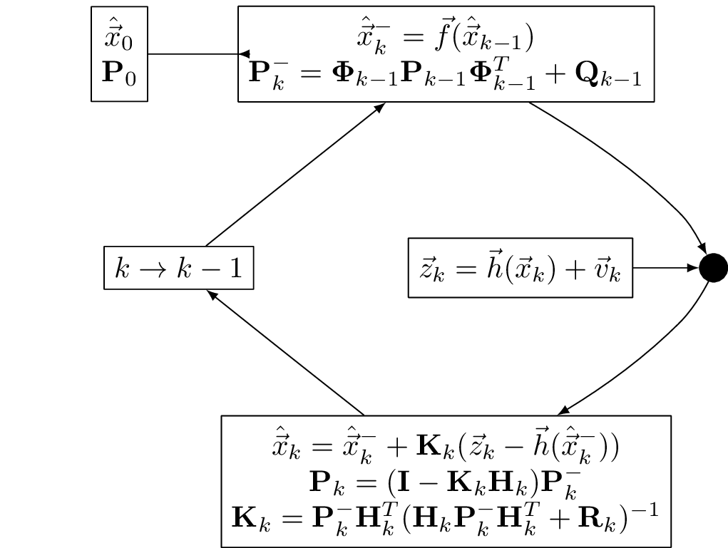
Extended Kalman Filter (EKF)
Write the linearized measurement as \[ \vec{z} - \vec{h}(\vec{x}^*) = \mathbf{H} \Delta \vec{x} + \vec{v} \] The incremental estimate update at time \(t_k\) is \[ \Delta\hat{\vec{x}}_k = \Delta\hat{\vec{x}}_k^- + \mathbf{K}_k \left[ \vec{z}_k - \vec{h}(\vec{x}^*_k) - \mathbf{H}_k \Delta\hat{\vec{x}}_k^- \right] \] Write the estimate of what the measurement should be \[ \hat{\vec{z}}^-_k = \vec{h}(\vec{x}^*_k) + \mathbf{H}_k \Delta\hat{\vec{x}}_k^- \] And then \[ \underbrace{\vec{x}^*_k + \Delta\hat{\vec{x}}_k}_{\textstyle\hat{\vec{x}}_k} = \underbrace{\vec{x}^*_k + \Delta\hat{\vec{x}}_k^-}_{\textstyle\hat{\vec{x}}_k^-} + \mathbf{K}_k \left[ \vec{z}_k - \hat{\vec{z}}^-_k \right] \]
EKF data flow
Pinson-9 model for inertial navigation
(Titterton and Weston 2004), (Raquet 2021)
Pinson 9-state model for INS is: \[ \vec{x} = \begin{bmatrix} \delta x_n \\ \delta x_e \\ \delta x_d \\ \delta v_n \\ \delta v_e \\ \delta v_d \\ \delta\epsilon_n \\ \delta\epsilon_e \\ \delta\epsilon_d \\ \end{bmatrix} = \begin{bmatrix} \delta\vec{x} \\ \delta\vec{v} \\ \delta\vec{\epsilon} \\ \end{bmatrix} \]
Where:
- \(\delta\vec{x}\) are the NED position error states
- \(\delta\vec{v}\) are the NED velocity error states
- \(\delta\vec{\epsilon}\) are the angle atittude errors
and \[
\dot{\vec{x}} = \mathbf{F} \vec{x}
\]
Imprantly \(\mathbf{F}\) is a matrix, this is not non-linear propagation.
Pinson-9 model propagation
\[ \begin{bmatrix} \delta\dot{\vec{x}} \\ \delta\dot{\vec{v}} \\ \delta\dot{\vec{\epsilon}} \end{bmatrix} = \begin{bmatrix} F_{xx} & F_{xv} & F_{x\epsilon} \\ F_{vx} & F_{vv} & F_{v\epsilon} \\ F_{\epsilon x} & F_{\epsilon v} & F_{\epsilon \epsilon} \\ \end{bmatrix} \begin{bmatrix} \delta \vec{x} \\ \delta \vec{v} \\ \delta \vec{\epsilon} \\ \end{bmatrix} \] We are working in geodetic coordinates so the elements of \(\mathbf{F}\) depend upon Earth specifc parameters to account for Coriolis force.
Pinson-9 model propagation definitions
| Variable | Description | Value/Units |
|---|---|---|
| \(\phi\) | latitude | radian |
| \(v_n\) | north velocity | meter/second |
| \(v_e\) | east velocity | meter/second |
| \(v_d\) | down velocity | meter/second |
| \(f_n\) | north specific force | meter/second/second |
| \(f_e\) | east specific force | meter/second/second |
| \(f_d\) | down specific force | meter/second/second |
| \(R_{\oplus}\) | Earth radius | 635300 meter |
| \(\Omega_{\oplus}\) | Earth rotation rate | 7.2921151467e-5/second |
Components of \(\mathbf{F}\), \(F_x\) row
\[ F_{xx} = \begin{bmatrix} 0 & 0 & -\frac{v_n}{R_{\oplus}^2}\\ \frac{v_e \tan \phi}{R_{\oplus}\cos \phi} & 0 & \frac{v_e}{R_{\oplus}^2 \cos\phi} \\ 0 & 0 & 0 \\ \end{bmatrix} \]
\[ F_{xv} = \begin{bmatrix} \frac{1}{R_{\oplus}} & 0 & 0\\ 0 & \frac{1}{R_{\oplus}\cos\phi} & 0 \\ 0 & 0 & -1 \\ \end{bmatrix} \]
\[ F_{x\epsilon} = \mathbf{0}_{3\times 3} \]
\(F_v\) row of \(\mathbf{F}\)
\[ F_{vx} = \begin{bmatrix} v_e \left( 2\Omega_{\oplus}\cos\phi + \frac{v_e}{R_{\oplus}\cos^2\phi} \right) & 0 & \frac{v_e^2\tan\phi - v_n v_d}{R_{\oplus}^2}\\ 2\Omega_{\oplus}\left(v_n \cos\phi - v_d \sin\phi\right) + \frac{v_n v_e}{R_{\oplus}\cos^2\phi} & 0 & \frac{-v_e (v_n\tan\phi +v_d)}{R_{\oplus}^2}\\ 2\Omega_{\oplus}v_e \sin \phi & 0 & \frac{v_n^2 + v_e^2}{R_{\oplus}} \\ \end{bmatrix} \]
\[ F_{vv} = \begin{bmatrix} \frac{v_d}{R_{\oplus}} & -2 \left( \Omega_{\oplus}\sin\phi + \frac{v_e\tan\phi}{R_{\oplus}} \right) & \frac{v_n}{R_{\oplus}} \\ 2\Omega_{\oplus}\sin\phi + \frac{v_e\tan\phi}{R_{\oplus}} & \frac{v_n\tan\phi+v_d}{R_{\oplus}} & 2\Omega_{\oplus}\cos\phi + \frac{v_e}{R_{\oplus}} \\ -\frac{2v_n}{R_{\oplus}} & -2 \left( \Omega_{\oplus}\cos\phi + \frac{v_e}{R_{\oplus}} \right) & 0 \\ \end{bmatrix} \]
\[ F_{v\epsilon} = \begin{bmatrix} 0 & -f_d & f_e \\ f_d & 0 & -f_n \\ -f_e & f_n & 0 \end{bmatrix} \]
\(F_\epsilon\) row of \(\mathbf{F}\)
\[ F_{\epsilon x} = \begin{bmatrix} -\Omega_{\oplus}\sin\phi & 0 & -\frac{v_e}{R_{\oplus}} \\ 0 & 0 & \frac{v_n}{R_{\oplus}^2} \\ -\Omega_{\oplus}\cos\phi - \frac{v_e}{R_{\oplus}\cos^2\phi} & 0 & \frac{v_e\tan\phi}{R_{\oplus}^2} \end{bmatrix} \]
\[ F_{\epsilon v } = \begin{bmatrix} 0 & 1/R_{\oplus}& 0 \\ -1/R_{\oplus}& 0 & 0 \\ 0 & \frac{\tan\phi}{R_{\oplus}} & 0 \\ \end{bmatrix} \]
\[ F_{\epsilon\epsilon} = \begin{bmatrix} 0 & -\Omega_{\oplus}\sin\phi + \frac{v_e}{R_{\oplus}\tan\phi} & v_n/R_{\oplus}\\ \Omega_{\oplus}\sin\phi + \frac{v_e\tan\phi}{R_{\oplus}} & 0 & \Omega_{\oplus}\cos\phi + v_e/R_{\oplus}\\ -v_n/R_{\oplus}& -\Omega\cos\phi -v_e/R_{\oplus}& 0 \\ \end{bmatrix} \]
Pinson-15 state model
- Extends the 9-state model to include
- accelerometer \(\vec{b_a}\) and gyro \(\vec{b_g}\) biases
- using First Order Gauss Markov model (FOGM)
\[ \vec{x} = \begin{bmatrix} \delta x_n \\ \delta x_e \\ \delta x_d \\ \delta v_n \\ \delta v_e \\ \delta v_d \\ \delta\epsilon_n \\ \delta\epsilon_e \\ \delta\epsilon_d \\ b_{a_x} \\ b_{a_y} \\ b_{a_z} \\ b_{g_x} \\ b_{g_y} \\ b_{g_z} \\ \end{bmatrix} = \begin{bmatrix} \delta\vec{x} \\ \delta\vec{v} \\ \delta\vec{\epsilon} \\ \vec{b_a}\\ \vec{b_g}\\ \end{bmatrix} \]
Propagation for 15-state Pinson model
\[ \begin{bmatrix} \delta\dot{\vec{x}} \\ \delta\dot{\vec{v}} \\ \delta\dot{\vec{\epsilon}} \\ \dot{\vec{b_a}}\\ \dot{\vec{b_g}}\\ \end{bmatrix} = \begin{bmatrix} F_{xx} & F_{xv} & 0 & 0 & 0\\ F_{vx} & F_{vv} & F_{v\epsilon} & \mathbf{C}_b^n & 0 \\ F_{\epsilon x} & F_{\epsilon v} & F_{\epsilon \epsilon} & 0 & -\mathbf{C}_b^n \\ 0 & 0 & 0 & F_{aa} & 0 \\ 0 & 0 & 0 & 0 & F_{gg} \\ \end{bmatrix} \begin{bmatrix} \delta \vec{x} \\ \delta \vec{v} \\ \delta \vec{\epsilon} \\ \vec{b}_a\\ \vec{b}_g\\ \end{bmatrix} \]
\[ F_{aa} = \begin{bmatrix} -1/\tau_a & 0 & 0 \\ 0 & -1/\tau_a & 0 \\ 0 & 0 & -1/\tau_a\\ \end{bmatrix},\ F_{gg} = \begin{bmatrix} -1/\tau_g & 0 & 0 \\ 0 & -1/\tau_g & 0 \\ 0 & 0 & -1/\tau_g\\ \end{bmatrix} \] and \(\mathbf{C}_b^n\) is the direction cosine matrix that rotates from body to NED frame.
MagNav additions to Pinson-15
- Add a barometer altimeter to constrain altitude
- \(\delta h_a\) is the altitude error correction to the INS
- \(\delta a\) is the vertical acceleration error (we already have \(\delta v_n\) in Pinson-9)
- Add a state \(S\) to model external time-correlated magnetic field variations
- disturbance field e.g. diurnal variations
- effects must be out-side of navigation frequency band
Results in an 18-component state vector \[ \begin{bmatrix} \delta \vec{x} & \delta \vec{v} & \delta \vec{\epsilon} & \vec{b}_a & \vec{b}_g & \delta h_a & \delta a & S \end{bmatrix} \]
Updates to \(\mathbf{F}\) matrix
\[ \begin{bmatrix} \delta\dot{\vec{x}} \\ \delta\dot{\vec{v}} \\ \delta\dot{\vec{\epsilon}} \\ \dot{\vec{b}}_a\\ \dot{\vec{b}}_g\\ \dot{h_a}\\ \dot{\delta_a}\\ \dot{S} \end{bmatrix} = \begin{bmatrix} F_{xx} & F_{xv} & 0 & 0 & 0 & F_{xb} & 0 \\ F_{vx} & F_{vv} & F_{v\epsilon} & \mathbf{C}_b^n & 0 & F_{vb} & 0 \\ F_{\epsilon x} & F_{\epsilon v} & F_{\epsilon \epsilon} & 0 & -\mathbf{C}_b^n & 0 & 0 \\ 0 & 0 & 0 & F_{aa} & 0 & 0 & 0\\ 0 & 0 & 0 & 0 & F_{gg} &0 & 0 \\ F_{bp} & 0 & 0 & 0 & 0 & F_{bb} & 0 \\ 0 & 0 & 0 & 0 & 0 & 0 & F_{ss} \\ \end{bmatrix} \begin{bmatrix} \delta \vec{x} \\ \delta \vec{v} \\ \delta \vec{\epsilon} \\ \vec{b}_a\\ \vec{b}_g\\ \delta h_a \\ \delta a \\ S \end{bmatrix} \]
Updated \(\mathbf{F}\) components
Barometer aiding: \[ \mathbf{F}_{xb} = \begin{bmatrix} 0 & 0 \\ 0 & 0 \\ k_1 & 0 \end{bmatrix},\ \mathbf{F}_{vb} = \begin{bmatrix} 0 & 0 \\ 0 & 0 \\ -k_2 & 1 \\ \end{bmatrix} \]
\[ \mathbf{F}_{bx} = \begin{bmatrix} 0 & 0 & 0\\ 0 & 0 & k_3 \\ \end{bmatrix},\ \mathbf{F}_{bb} = \begin{bmatrix} -\frac{1}{\tau_b} & 0 \\ -k_3 & 0 \\ \end{bmatrix} \]
The disturbance field bias is given by: \[ \mathbf{F}_{ss} = \frac{1}{\tau_s} \]
MagNav measurement processor
The scalar sensor measures: \[ |\vec{B}_\text{total}| = |\vec{B}_\text{ext}+ \vec{B}_\text{\class{fa fa-plane}{}} | \] and \[ \vec{B}_\text{ext}= \vec{B}_{\oplus}+ \vec{B}_\text{anomaly} + \vec{B}_\text{disturbance} \]
- We added a state \(S\) into the MagNav model to account for \(\vec{B}_\text{disturbance}\).
- \(\vec{B}_{\oplus}\) from IGRF or WMM
- Both IGRF and WMM are functions of lat, long, altitude and time
- WMM has \(28.8^\circ\) or 3200 km at surface resolution
- Secular variaton \(\approx 100 \text{nT}/\text{year} = 0.27 \text{nT}/\text{day}\)
MagNav Measurement Processor \(H\) matrix
\[ \begin{aligned} \vec{z} & \approx \vec{h}(\vec{x}^*, t) + \mathbf{H} \cdot \Delta\vec{x} + \vec{v}(t) \end{aligned} \]
\[ \mathbf{H} = \left[ \frac{\partial \vec{h}}{\partial \vec{x}}\right]_{\vec{x}=\vec{x}^*} \]
\[ \mathbf{H}(\vec{x}^*) = \begin{bmatrix} \frac{\partial h(\vec{x}^*)}{\partial x_n} \\ \frac{\partial h(\vec{x}^*)}{\partial x_e} \\ \frac{\partial h(\vec{x}^*)}{\partial x_d} \\ \mathbf{0}_{1x15} \end{bmatrix} \leftarrow\text{This is the gradient of the map} \] Both the map and 3D gradient of the map are needed in order to make a measurement and incorporate it.
Simplified sequential processing
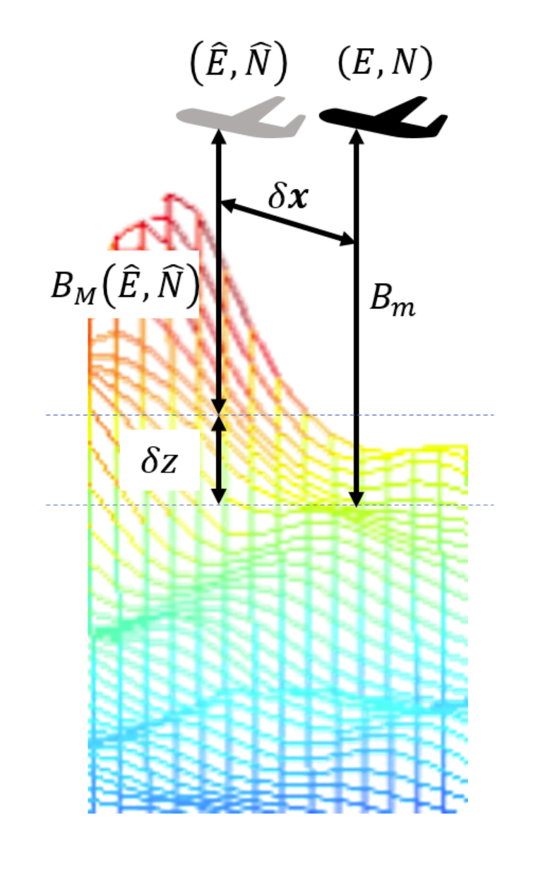
- Measurement processor: \(\delta z = B_\text{measured} - B_\text{map}(\hat{E},\hat{N})\)
- \(B_\text{measured}\) is measured magnetic field
- \(B_\text{map}(\hat{E},\hat{N})\) is the predicted map value based on position estimate
- State vector error: \(\delta \vec{x} = \left[ \delta E, \delta N \right]^T\)
- Measurement matrix: \(\mathbf{H} = \left[ \frac{\partial B_\text{map}(\hat{E},\hat{N})}{\partial E} \frac{\partial B_\text{map}(\hat{E},\hat{N})}{\partial N} \right]\)
- Measurement equation: \(\mathbf{H} \delta \vec{x}\)
- Update of the state vector error depends on the map gradients in East and North directions
Navigation pre-processor
- Prepare Magnetic Anomaly Map
- Upward continue as needed for flight altitudes
- Compute 3-D gradient for measurement processor
- Precompute Core field model as needed
- Prepare Tolles-Lawson Compensation coefficients
- In an adaptive or online calibration this is a starting point
Filter initialization
- Assume known starting value for position and attitude from GPS-aided system
- Tolles-Lawson coefficients are needed
- Works well for EKF - provides excellent starting point for state
- State starting point initializes map error state \(S\)
Wrapup
Wrapup
- Real-world demonstrations
- Discussion
- Social hour(s)
Real world examples
- Geophysical survey aircraft
- T-38
- F-16
- C-17
- Commercial E-170 and AW-139
Survey aircraft
T-38
F-16
F-16 photos approved for public release by Edwards AFB Public Affairs Office. Public Release number 20438.
C-17
Honeywell
Discussion
Social following workshop
Please join us at Salty Seal Brewpub
Salty Seal Brewpub and Sports Bar
653 Cannery Row, Monterey, CA 93940
5-8pm
References

ION MagNav Workshop 2023


 From
From 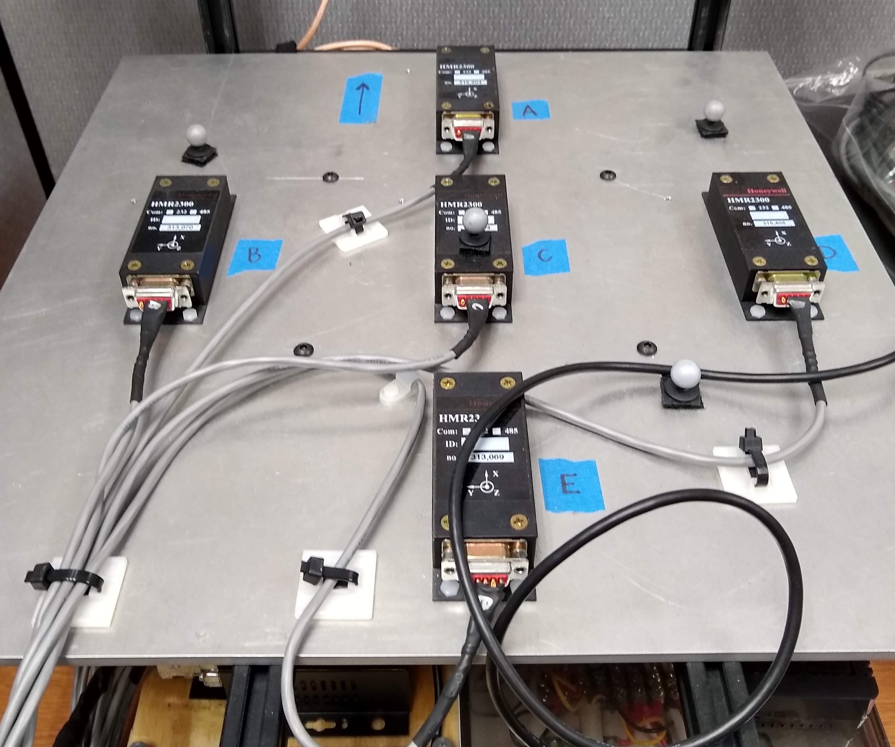






Social