Compensation and Calibration

ION MagNav Workshop 2023, Monterey, CA

Aaron Nielsen

The views expressed in this article are those of the author and do not necessarily reflect the official policy or position of the United States Government, Department of Defense, United States Air Force or Air University.

Distribution A: Authorized for public release. Distribution is unlimited. Case No. 2023-0427.

https://rpubs.com/friendly/test-newcommands https://quarto.org/docs/authoring/markdown-basics.html#equations

https://stackoverflow.com/questions/41362012/how-to-insert-font-awesome-icons-in-mathjax

Font-Awesome will only work for html type output

$$

$$

Traditional Tolles-Lawson calibration

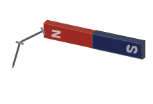
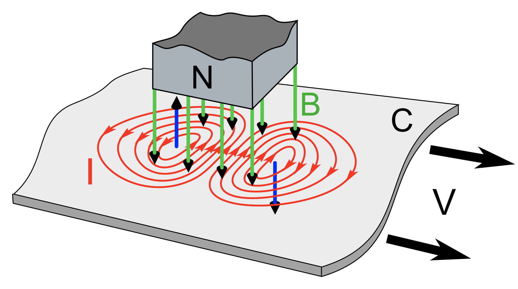
An airplane is a big magnet that flies

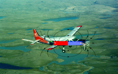
\(|\vec{B}_\text{sensor}| = |\vec{B}_{\oplus}+ \vec{B}_\text{anomaly}+ \vec{B}_\text{disturbance}+ \vec{B}_\class{fa fa-plane}{}|\)

An airplane is a big magnet that flies

\(|\vec{B}_\text{sensor}| = |\vec{B}_{\oplus}+ \vec{B}_\text{anomaly}+ \vec{B}_\text{disturbance}+ \vec{B}_\class{fa fa-plane}{}|\)

\(|\vec{B}_\text{ext}| = |\vec{B}_{\oplus}+ \vec{B}_\text{anomaly} + \vec{B}_\text{disturbance}|\)

\(|\vec{B}_\text{sensor}| = |\vec{B}_\text{ext}+ \vec{B}_\class{fa fa-plane}{}|\)

assume \(|\vec{B}_\class{fa fa-plane}{}|/|\vec{B}_\text{ext}|\ll 1\)

\(|\vec{B}| \approx |\vec{B}_\text{ext}| + \frac{1}{2}\vec{B}_\class{fa fa-plane}{}\cdot\vec{B}_\text{ext}\)

need a model for \(\vec{B}_\class{fa fa-plane}{}\)

(Gnadt 2022)

Tolles-Lawson

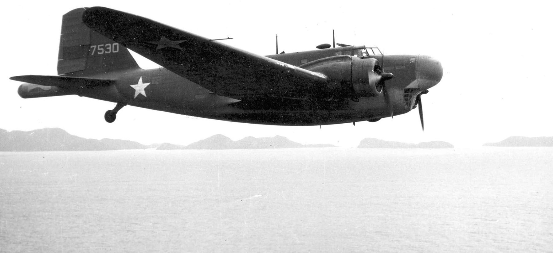
• Calibration technique developed in WW2 for submarine hunting
• Declassified in 1950’s and patented
• Standard calibration technique used for aero-magnetic surveys
  • Developed by (Leliak 1961)

\[ \begin{align*} |B_\text{sensor}| &= |\vec{B}_\text{ext}+ \vec{B}_\class{fa fa-plane}{}|\\ &= \sqrt{ |B_\text{ext}|^2 + |B_\class{fa fa-plane}{}|^2 + 2 |B_\text{ext}||B_\class{fa fa-plane}{}|\cos\theta}\\ |B_\text{sensor}| &= |B_\text{ext}| \sqrt{ 1 + \frac{|B_\class{fa fa-plane}{}|^2}{|B_\text{ext}|^2} + 2\frac{|B_\class{fa fa-plane}{}|}{|B_\text{ext}|}\cos\theta} \end{align*} \]

Tolles-Lawson

• Calibration technique developed in WW2 for submarine hunting
• Declassified in 1950’s and patented
• Standard calibration technique used for aero-magnetic surveys
  • Developed by (Leliak 1961)

\[ \begin{align*} |B_\text{sensor}| &= |\vec{B}_\text{ext}+ \vec{B}_\class{fa fa-plane}{}|\\ &= \sqrt{ |B_\text{ext}|^2 + |B_\class{fa fa-plane}{}|^2 + 2 |B_\text{ext}||B_\class{fa fa-plane}{}|\cos\theta}\\ |B_\text{sensor}| &= |B_\text{ext}| \sqrt{1 + 2\frac{|B_\class{fa fa-plane}{}|}{|B_\text{ext}|}\cos\theta} \end{align*} \]

Tolles-Lawson Path to Calibration 1/2

\[ \begin{align*} |B_\text{Sensor}| &= |\vec{B}_\text{ext}+ \vec{B}_\class{fa fa-plane}{}|\\ &= \sqrt{ |B_\text{ext}|^2 + |B_\class{fa fa-plane}{}|^2 + 2 |B_\text{ext}||B_\class{fa fa-plane}{}|\cos\theta}\\ |B_\text{Sensor}| &= |B_\text{ext}| \sqrt{ 1 + 2\frac{|B_\class{fa fa-plane}{}|}{|B_\text{ext}|}\cos\theta}\\ &\approx |B_\text{ext}| + |B_\class{fa fa-plane}{}|\cos\theta + \cdots \end{align*} \]

Path to Calibration
Measure \(\cos\theta\)

Solve \(|B_\text{sensor}| = |B_\text{ext}| + |B_\class{fa fa-plane}{}|\cos\theta\)

Assuming \(|B_\text{ext}|\) is known or constant

Tolles-Lawson Path to Calibration 2/2

Path to Calibration
Measure \(\cos\theta\)

Solve \(|B_\text{sensor}| = |B_\text{ext}| + |B_\class{fa fa-plane}{}|\cos\theta\)

Assuming \(|B_\text{ext}|\) is known or constant


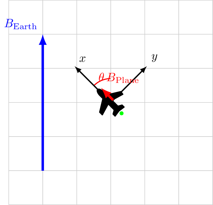
How to measure \(\cos\theta\)?
Use a vector magnetometer

Rotate aircraft in \(\vec{B}_\text{ext}\)

Direction cosines

• The direction cosines are computed in the vector magnetometer reference frame
• The magnetometer is fixed to aircraft body reference frame \[ \begin{aligned} \cos X = & \frac{B_x}{\sqrt{B_x^2 + B_y^2 + B_z^2}}\\ \cos Y = & \frac{B_y}{\sqrt{B_x^2 + B_y^2 + B_z^2}}\\ \cos Z = & \frac{B_z}{\sqrt{B_x^2 + B_y^2 + B_z^2}} \end{aligned} \]

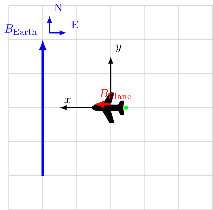
Calibration 1/4

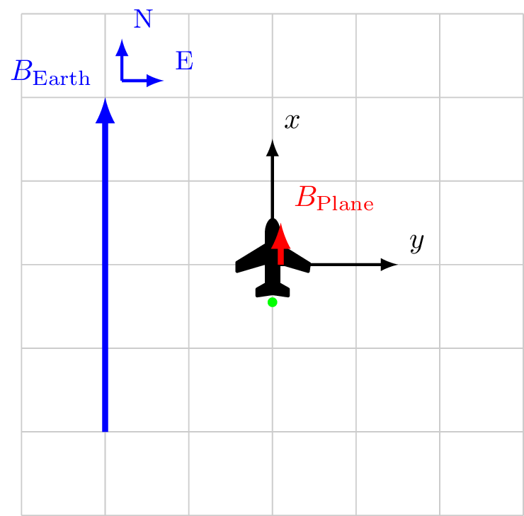
Coordinate system fixed to aircraft
\[\vec{B}_\text{Sensor} = \vec{B}_\text{ext}+ \vec{B}_\class{fa fa-plane}{}\]
\[ \begin{alignat*}{3} \vec{B}_\text{ext}&= 4.0 \hat{x} && + 0.0 \hat{y} \\ \vec{B}_\class{fa fa-plane}{}&= 0.5 \hat{x} && +0.0 \hat{y} \\ \vec{B}_\text{Sensor} &= 4.5 \hat{x} && + 0.0 \hat{y} \\ |B_\text{Sensor}| &= 4.5 && \\ \cos X &= \frac{4.5}{4.5} && = 1\\ \cos Y &= \frac{0.0}{4.5} && = 0\\ \end{alignat*} \]

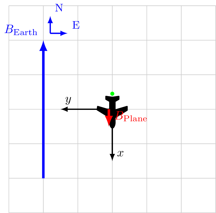
Calibration 2/4

Coordinate system fixed to aircraft
\[\vec{B}_\text{Sensor} = \vec{B}_\text{ext}+ \vec{B}_\class{fa fa-plane}{}\]
\[ \begin{alignat*}{3} \vec{B}_\text{ext}&= 0.0 \hat{x} && + 4.0 \hat{y} \\ \vec{B}_\class{fa fa-plane}{}&= 0.5 \hat{x} && + 0.0 \hat{y} \\ \vec{B}_\text{Sensor} &= 0.5 \hat{x} && + 4.0 \hat{y} \\ |B_\text{Sensor}| &= 4.007 && \\ \cos X &= \frac{0.5}{4.007} && \ne 0 \rightarrow 82.8^\circ\\ \cos Y &= \frac{4.0}{4.007} && \approx 1\\ \end{alignat*} \]

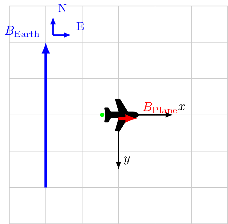
Calibration 3/4

Coordinate system fixed to aircraft
\[\vec{B}_\text{Sensor} = \vec{B}_\text{ext}+ \vec{B}_\class{fa fa-plane}{}\]
\[ \begin{alignat*}{3} \vec{B}_\text{ext}&= -4.0 \hat{x} && + 0.0 \hat{y} \\ \vec{B}_\class{fa fa-plane}{}&= 0.5 \hat{x} && + 0.0 \hat{y} \\ \vec{B}_\text{Sensor} &= -3.5 \hat{x} && + 0.0 \hat{y} \\ |B_\text{Sensor}| &= 3.5 && \\ \cos X &= \frac{-3.5}{3.5} && = -1\\ \cos Y &= \frac{0}{3.5} && = 0\\ \end{alignat*} \]

Calibration 4/4

Coordinate system fixed to aircraft
\[\vec{B}_\text{Sensor} = \vec{B}_\text{ext}+ \vec{B}_\class{fa fa-plane}{}\]
\[ \begin{alignat*}{3} \vec{B}_\text{ext}&= 0.0 \hat{x} && + -4.0 \hat{y} \\ \vec{B}_\class{fa fa-plane}{}&= 0.5 \hat{x} && + 0.0 \hat{y} \\ \vec{B}_\text{Sensor} &= 0.5 \hat{x} && + -4.0 \hat{y} \\ |B_\text{Sensor}| &= 4.007 &&\\ \cos X &= \frac{0.5}{4.007} && \ne 0\\ \cos Y &= \frac{-4.0}{4.007} && \approx -1\\ \end{alignat*} \]

Standard calibration model - Tolles-Lawson

\[|\vec{B}_\text{sensor}| = |\vec{B}_\text{ext}+ \vec{B}_\class{fa fa-plane}{}|\]

\[ \begin{array}{ l B c B c B c } \vec{B}_\class{fa fa-plane}{}& = & \vec{B}_\text{Permanent} & + & \vec{B}_\text{Induced} & + & \vec{B}_\text{Eddy}\\ & = & \vec{P}_\text{constant} {} & + &{} M_{3\times3} \vec{B}_\text{ext}{} & + & {} S_{3\times3} \frac{\partial}{\partial t} \vec{B}_\text{ext} \end{array} \]

\(M_{3\times3}\) is symmetric \(\rightarrow\) 6 independent elements

Total of 18 elements

Use the same direction cosines, now with \(B_z\)

The direction cosines are computed from the vector magnetometer

\[ \begin{aligned} \cos X = & \frac{B_x}{\sqrt{B_x^2 + B_y^2 + B_z^2}}\\ \cos Y = & \frac{B_y}{\sqrt{B_x^2 + B_y^2 + B_z^2}}\\ \cos Z = & \frac{B_z}{\sqrt{B_x^2 + B_y^2 + B_z^2}} \end{aligned} \]

Tolles-Lawson full implementation

\[ \begin{aligned} B_\class{fa fa-plane}{}& = & & { c_1 \cos X + c_2 \cos Y + c_3 \cos Z }+ \\ & & B_\text{ext}& {[ c_4 \cos^2 X + c_5 \cos X \cos Y + c_6 \cos X \cos Z +} \\ & & & { c_7 \cos^2 Y + c_8 \cos Y \cos Z + c_9 \cos^2 Z ] + } \\ & & B_\text{ext}& { [ c_{10} \cos X \cos' X + c_{11} \cos X \cos' Y + c_{12} \cos X \cos' Z }+ \\ & & & { c_{13} \cos Y \cos' X + c_{14} \cos Y \cos' Y + c_{15} \cos Y \cos' Z +} \\ & & & { c_{16} \cos Z \cos' X + c_{17} \cos Z \cos' Y + c_{18} \cos Z \cos' Z ] } \end{aligned} \]
- We need a method to solve for \(c_1 \ldots c_{18}\) - Should provide visibility over anticipated range of aircraft motion

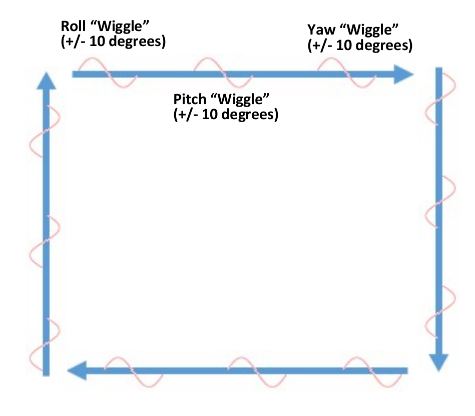
Calibration manuevers - Tolles-Lawson

Fly the aircraft in a series of Roll, Pitch, Yaw maneuvers

• High-altitude

• Altitude of a known map

Maneuver angle should depend upon the expected aircraft dynamics

• Barrel Rolls?

Typically at each cardinal heading

• 3 rolls \(\pm 10^\circ\) at 1 Hz
• 3 pitches \(\pm 10^\circ\) at 1 Hz
• 3 yaws \(\pm 10^\circ\) at 1 Hz

(W. E. Tolles and Lawson 1950), (W. E. Tolles 1954), (W. E. Tolles 1955), (Gnadt, Wollaber, and Nielsen 2022)

Construct Tolles-Lawson \(A\) matrix

\[ A = \begin{bmatrix} \cos X_1 & \cdots & \cos X_N\\ \cos Y_1 & \cdots & \cos Y_N \\ \cos Z_1 & \cdots & \cos Z_N\\ B_\text{ext}\cos^2 X_1 & \cdots & B_\text{ext}\cos^2 X_N\\ B_\text{ext}\cos X_1 \cos Y_1 & \cdots & B_\text{ext}\cos X_N \cos Y_N\\ B_\text{ext}\cos X_1 \cos Z_1 & \cdots & B_\text{ext}\cos X_N \cos Z_N \\ B_\text{ext}\cos^2 Y_1 & \cdots & B_\text{ext}\cos^2 Y_N \\ B_\text{ext}\cos Y_1 \cos Z_1 & \cdots & B_\text{ext}\cos Y_N \cos Z_N\\ B_\text{ext}\cos^2 Z_1 & \cdots & B_\text{ext}\cos^2 Z_N\\ B_\text{ext}\cos X_1 \cos' X_1 & \cdots & B_\text{ext}\cos X_N \cos' X_N \\ B_\text{ext}\cos X_1 \cos' Y_1 & \cdots & B_\text{ext}\cos X_N \cos' Y_N\\ B_\text{ext}\cos X_1 \cos' Z_1 & \cdots & B_\text{ext}\cos X_N \cos' Z_N\\ B_\text{ext}\cos Y_1 \cos' X_1 & \cdots & B_\text{ext}\cos Y_N \cos' X_N\\ \vdots & & \vdots \\ B_\text{ext}\cos Z_1 \cos' Z_1 & \cdots & B_\text{ext}\cos Z_N \cos' Z_N \\ \end{bmatrix} \]

\(H_e\) is the magnitude of the external field. We assume that \[ B_\text{ext}= \sqrt{B_x^2 + B_y^2 + B_z^2} \]
Equivalently that the vector mags only see external field. The anomaly signal is below the noise floor.

Solve for the \(c_i\) coefficients

Map-less calibration
Perform maneuvers at fixed frequency \(f\)
Band-pass filter columns of \(A\), \(B_\text{scalar}\) \[ \begin{aligned} A_f & = BPF(A)\\ B_{\text{scalar},f} & = BPF(B_{\text{scalar}}) \end{aligned} \]
Solve for \(c\)

\[ A_f \cdot c = B_{\text{scalar},f} \]

Map-based calibration
Perform maneuvers over known-good map

Solve for \(c\)
\[ A \cdot c = B_{\text{scalar}} - B_{{\oplus}} - B_{\text{anomaly}} \]

Multi-colinearity in solution

• There is multi-colinearity in the A-matrix via two constraints
  • \(\cos^2 X + \cos^2 Y + cos^2 Z = 1\)
  • \(\cos' X \cos X + \cos' Y \cos Y + \cos'Z \cos Z = 0\)
• Solving \(A^T c^T = B_\class{fa fa-plane}{}\) is overdetermined
• The standard solution is ordinary least squares \[ \begin{aligned} Ac & = B_\class{fa fa-plane}{}\\ A^T A c & = A^T B_\class{fa fa-plane}{}\\ c & = (A^T A)^{-1} A^T B_\class{fa fa-plane}{} \end{aligned} \]
• This is effectively what numpy’s np.linalg.lstsq performs.
• Often this works just fine

Ridge regression

• If there is multi-colinearity, Ridge regression is one technique that can be used
• Solve inteads: \[c = \left( (A^T A+ kI)^{-1} A^T \right) B_\class{fa fa-plane}{}\]
• \(k\) is called the Ridge parameter since it’s along the diagonal and it should be small
  • \(k=0\) is standard linear regression
  • Otherwise must determine hyper-parameter \(k\)
• Python package scikit-learn provides Ridge and RidgeCV routines to do this

Ridge regression

• Ridge regression results generally less dependent upon small changes to the data
  • More robust to noisy data
• Goal of ridge regression is not to find the smallest error
• Goal is to find a solution that is less sensitive to small variations in input data
  • May produce a biased result

Finding ridge regression hyper-parameter \(k\)

• \(k \rightarrow \infty\) leads to \(c=0\)
• \(k = 0\) leads to regular least squares
• Examine “Ridge Trace” Plot
• Identify where the \(c\) stabilize

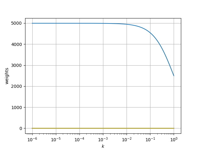
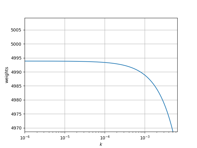
Finding ridge regression hyper-parameter \(k\)

• \(k \rightarrow \infty\) leads to \(c=0\)
• \(k = 0\) leads to regular least squares
• Examine “Ridge Trace” Plot
• Identify where the \(c\) stabilize
• In this case \(k\approx 1\times10^{-4}\)

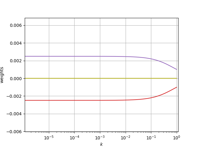
Finding ridge regression hyper-parameter \(k\)

• \(k \rightarrow \infty\) leads to \(c=0\)
• \(k = 0\) leads to regular least squares
• Examine “Ridge Trace” Plot
• Identify where the \(c\) stabilize
• In this case \(k\approx 1\times10^{-4}\)

Apply \(c\) to in-flight data for comparison

In-flight
Compute \(A_k\) for each time-step

Apply \(c\)

\[ B_\class{fa fa-plane}{}= A \cdot c \]
\[ B_\text{anomaly}= B_\text{sensor}- B_{\oplus}- B_\class{fa fa-plane}{} \]

References

Gnadt, Albert R. 2022. “Machine Learning-Enhanced Magnetic Calibration for Airborne Magnetic Anomaly Navigation.” In AIAA SciTech 2022 Forum. https://doi.org/10.2514/6.2022-1760.

Gnadt, Albert R., Allan B. Wollaber, and Aaron P. Nielsen. 2022. “Derivation and Extensions of the Tolles-Lawson Model for Aeromagnetic Compensation.” arXiv. https://doi.org/10.48550/ARXIV.2212.09899.

Leliak, Paul. 1961. “Identification and Evaluation of Magnetic-Field Sources of Magnetic Airborne Detector Equipped Aircraft.” IRE Transactions on Aeronautical and Navigational Electronics ANE-8 (3): 95–105. https://doi.org/10.1109/TANE3.1961.4201799.

Tolles, W E, and J D Lawson. 1950. “Magnetic compensation of MAD equipped aircraft.” Airborne Instruments Lab. Inc., Mineola, NY, Rept, 201–1.

Tolles, W. E. 1954. Compensation of aircraft magnetic fields. 2692970, issued 1954.

———. 1955. Magnetic field compensation system. 2706801, issued 1955.