Navigable map metrics

ION MagNav Workshop 2023, Monterey, CA

Aaron Nielsen

The views expressed in this article are those of the author and do not necessarily reflect the official policy or position of the United States Government, Department of Defense, United States Air Force or Air University.

Distribution A: Authorized for public release. Distribution is unlimited. Case No. 2023-0427.

Outline

https://rpubs.com/friendly/test-newcommands https://quarto.org/docs/authoring/markdown-basics.html#equations

https://stackoverflow.com/questions/41362012/how-to-insert-font-awesome-icons-in-mathjax

Font-Awesome will only work for html type output

$$

$$

Outline

• Aeromagnetic survey best practices
• Analysis of maps for navigation

Aeromagnetic survey practices for MagNav

• Tolles-Lawson calibration flown before and/or after survey
• Surveys usually flown in grid pattern
  • Flight lines used to model anomaly intensity
  • Tie lines used for map leveling
• Local ground magnetometer reference station
  • Records temporal changes of disturbance field
• (Bergeron and Nielsen 2023)

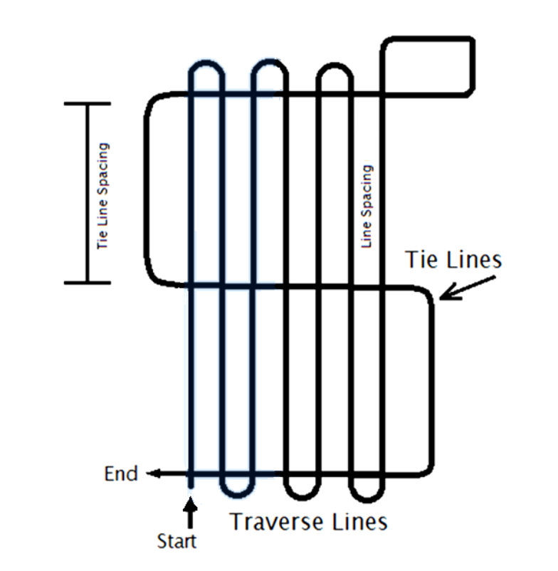
Example aeromagnetic survey flight path with dense, parallel flight lines and spare orthogonal tie lines.

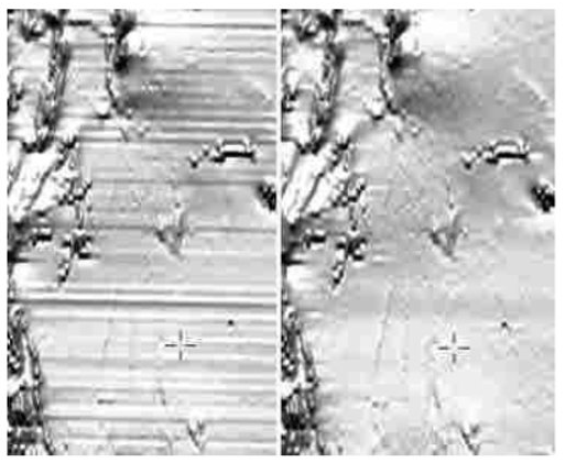
Heading error and corrugation

• Heading error results in corrugation
  • Mitigated via map leveling
    • Usually by minimizing flight/tie line intersection differences
    • (Reeves 2005), (Luyendyk 1997)

(Reeves 2005)

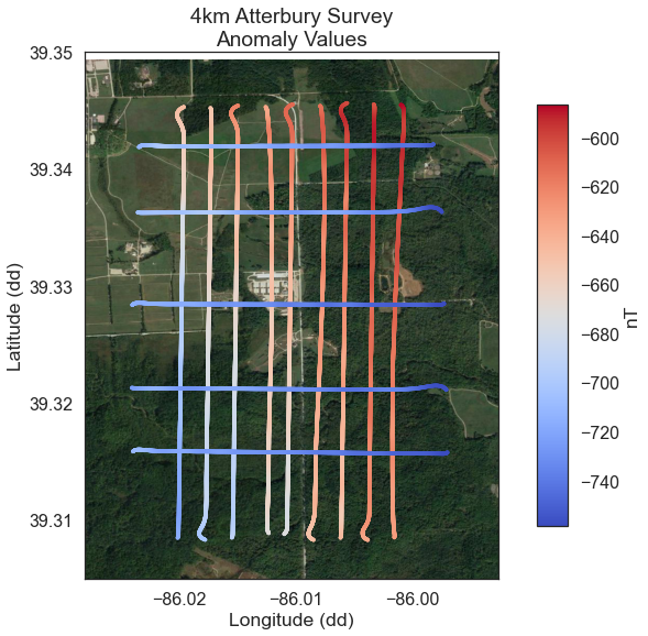
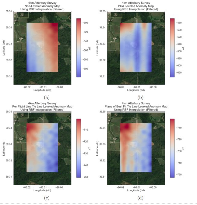
Differing leveling algorithms produce different results

(Bergeron and Nielsen 2023)

Corrugation figure of merit

• Used to determine map leveling effectiveness
• Process:
  • High-pass filter in the tie-line direction
    • cut-off frequency give by the survey altitude AGL
    • Average in flight line direction
    • Fourier transform of average
    • Largest magnitude within corrugation bandwidth (\(B_c\)) selected
      • \(B_c\) is the corrugation bandwidth
      • \(a_{agl}\) is the survey altitude
    • Invert magnitude value to obtain FOM
  • \[\frac{1}{a_{agl}(1+0.05)} \le B_c \le \frac{1}{a_{agl}(1+0.05)}\]

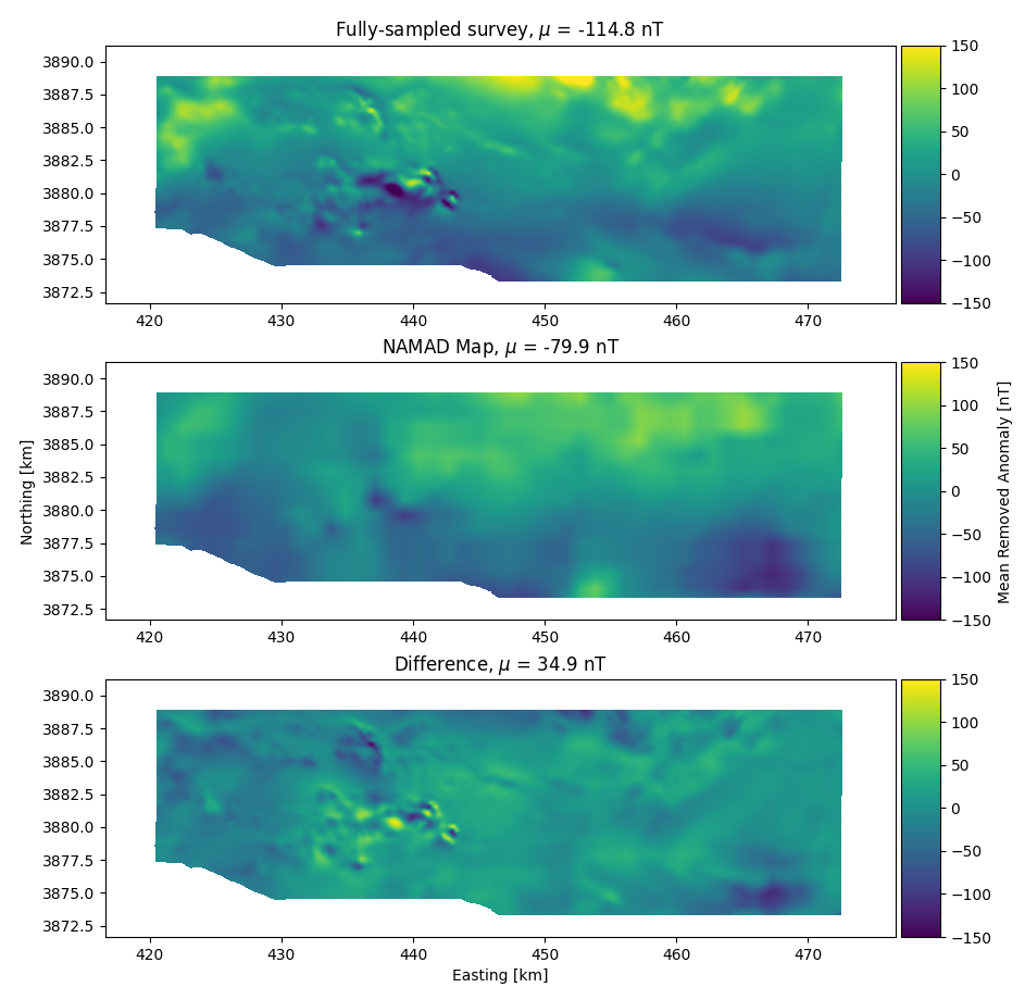
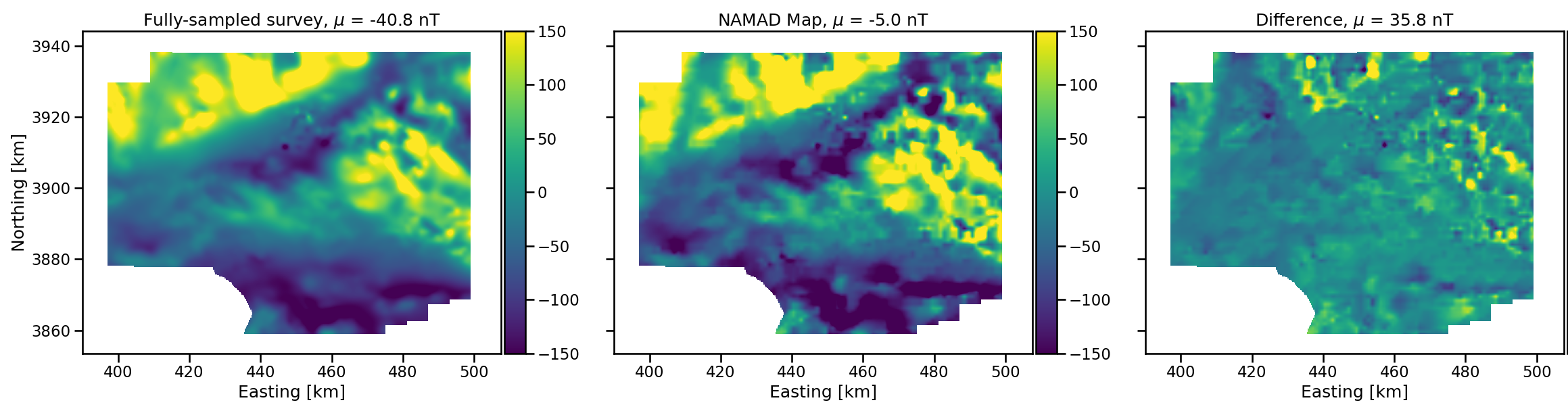
Map comparisons

• Magnetic maps of Mojave Desert
  • Both at 300 m above ground level
• NAMAD (Bankey et al. 2002)
  • resolution 1.1 km
• Fully sampled
  • resolution 75 m
• Obvious missing features in NAMAD

(Nielsen, Gray, and Bonifaz 2022)

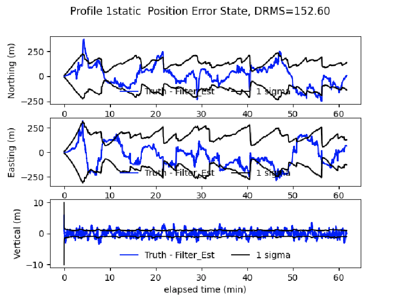
Navigation flight comparison - fully-sampled map

• Recent F-16 flight test demonstrated good navigation performance with a fully-sampled map
• Challenging calibration problem (\(\approx\) 5000 nT)
  • Believe this to be the limiting factor to navigation performance
• Typical DRMS errors \(\approx\) 150 m
• (Canciani 2021), (Bonifaz 2022)

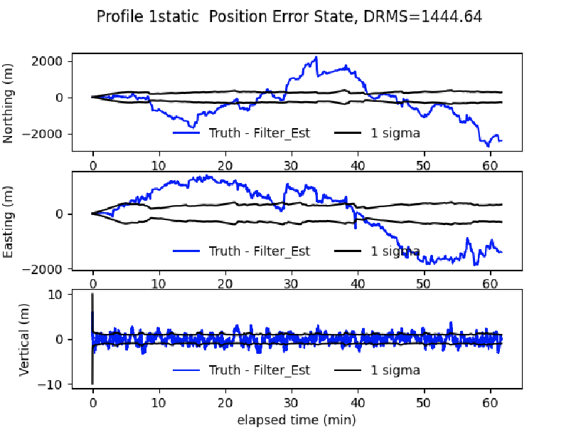
Navigation flight comparison - NAMAD map

• Substitute NAMAD map in navigator
• Typical DRMS errors \(\approx\) 1500 m
• Error grows \(\approx 10\times\)
• Only difference is the map used to navigate
  • NAMAD typical of existing surveys
• What features drive larger error?
• How are these features quantified?

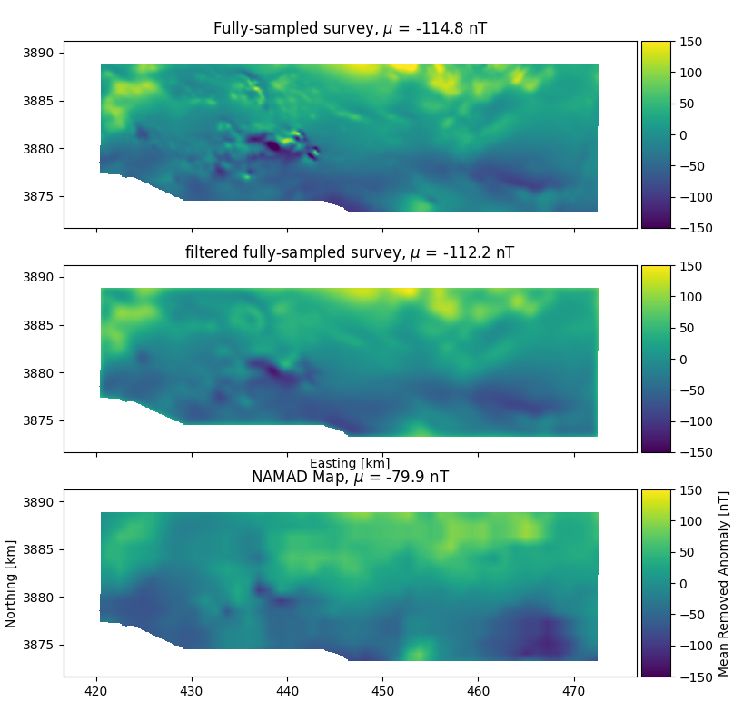
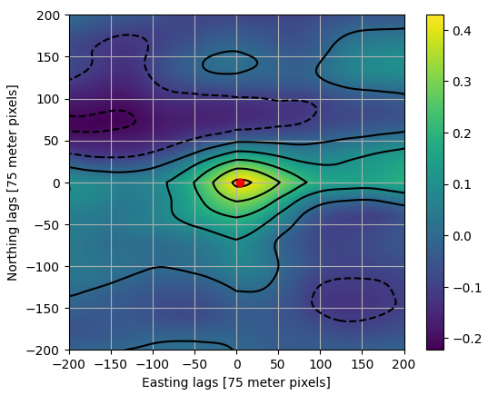
Map cross-correlation

• Filter fully-sampled map to NAMAD resolution
  • 1.1 km
• Planar detrend both maps and perform cross-correlation
• Overall shift of 700 m between maps

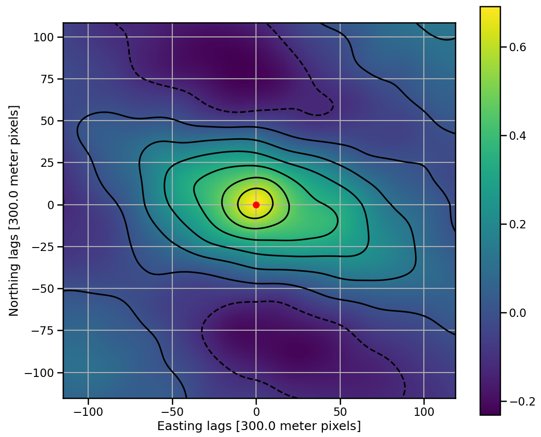
Cross-correlation with fully-sampled NAMAD

• NAMAD spatial resolution becomes fully sampled at \(\approx\) 1100 m AGL
• Fully-sampled map survey flown at 2133 m AGL
• No overall shift between maps
• Registration errors masked at fully-sampled altitude

Tiled cross-correlation

• Hypothesis:
  • Different regions of NAMAD need different translations to match real magnetic anomaly
  • Segmented the maps into small sections
• Cross-correlate each section
• Make a map of the cross-correlation results
  • Identify regions of different cross-correlation

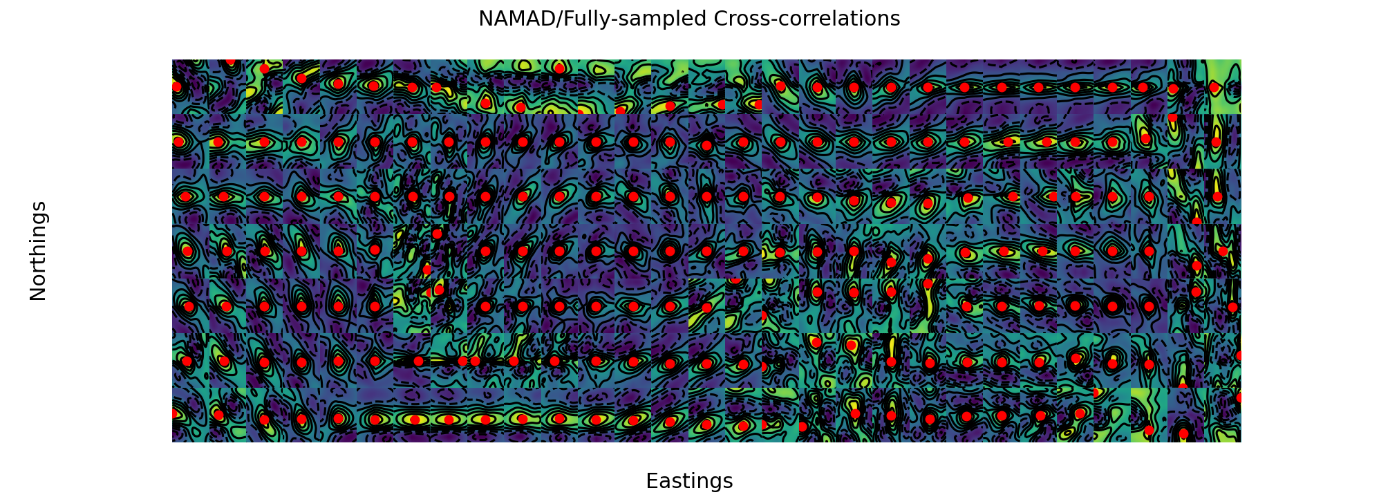
Tiled cross-correlation results

• Identify regions of different cross-correlation properties
  • specifically a shift is peak location
• Traversing from one region to another adds a shift to the navigation solution
• Breaks long-distance correlations

Underlying NAMAD data

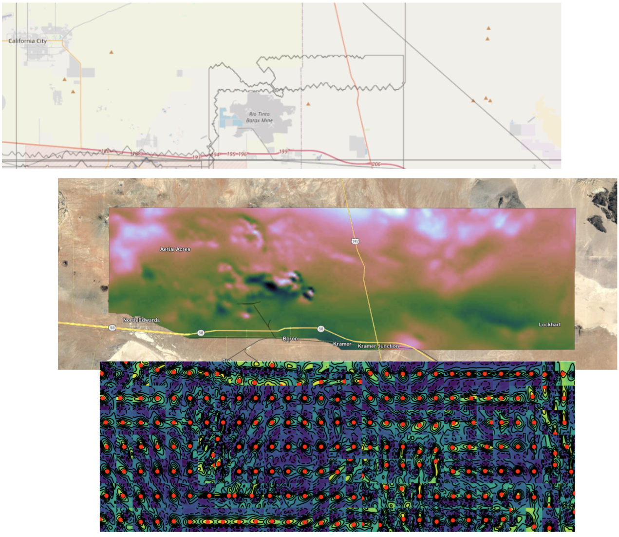
• Top Plot shows USGS survey boundaries (gray)
• Major feature in center Rio Tinto Borax Mine
  • Open pit mining began 1957
• Many USGS survey in area 1954, 1955, 1978 (NURE)
  • Oldest are hand-drawn digitized maps
• Survyes pre-date GPS
• Major cross-correlation peak shifts coincide with survey boundaries

Auto-correlation analysis

• NAMAD map auto-correlation differs in width and structure from fully-sampled map
  • Fully-sampled map is asymmetic and longer

Auto-correlation line cuts

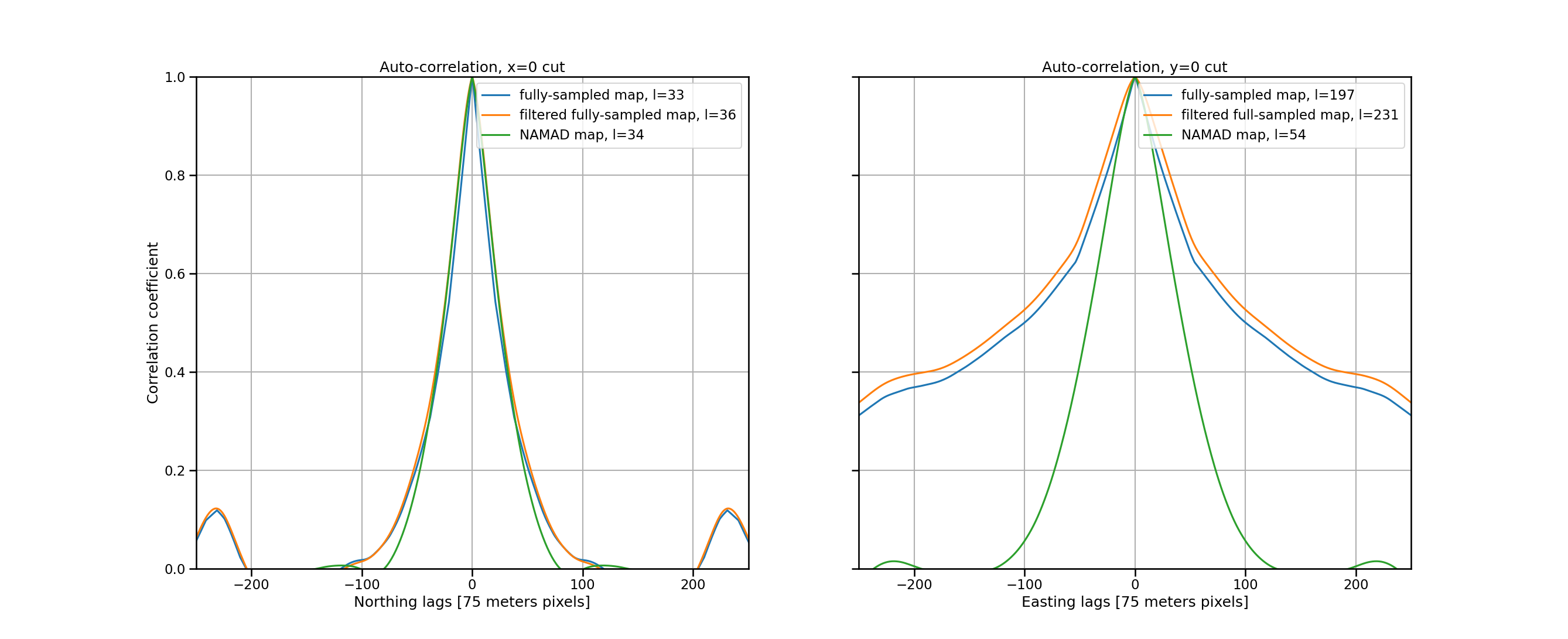
• Filtering to NAMAD spacing results in nearly same spatial correlation as unfiltered
• NAMAD map auto-correlation length
  • Easting \(\approx 4 \times\) smaller than fully-sampled map
  • Northing approx the same
• Geo-registration shifts in NAMAD cause loss of correlation

Power-spectral analysis

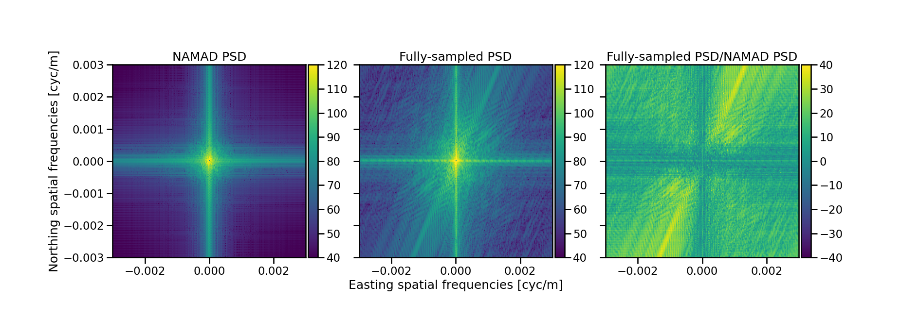
• NAMAD map confined to very narrow frequency reponse
• As much as 40 dB of energy missing at higher frequecies in NAMAD

Aircraft velocity translates spatial into temporal

• Vehicle velocity \(\vec{v}\) translates spatial magnetic anomaly into temporal anomaly
• Exponential autocorreltion length \(\ell\) in map becomes First Order Gauss-Markov process in magnetic sensor
  • \(\tau = \frac{\ell}{v}\)
• Spatial frequencies \(\vec{k}\) translate into temporal frequencies \(f\)
  • \(f = \vec{v} \cdot \vec{k}\)

• NAMAD auto-correlation lengths tranlsate to \(\tau\approx 30\ \text{second}\)
• F-16 Space-weather FOGM \(\tau\approx 30\ \text{second}\)
• Low-frequency map correlations accomondated by Nav filter FOGM
• High-frequency spatial content missing NAMAD
• Almost nothing left to navigate

References

Bankey, Viki, Alejandro Cuevas, David Daniels, Carol A. Finn, Israel Hernandez, Patricia Hill, Robert Kucks, et al. 2002. “Digital Data Grids for the Magnetic Anomaly Map of North America.” U.S. Department of the Interior, U.S. Geological Survey; Online; US Geological Survey. https://doi.org/10.3133/ofr02414.

Bergeron, Luke, and Aaron Nielsen. 2023. “Aeromagnetic Anomaly Mapping for Navigation.” In Proceedings of IEEE/ION PLANS 2023.

Bonifaz, Jonnathan. 2022. “Magnetic Navigation Using Online Calibration Filter Analysis.” Master’s thesis, Air Force Institute of Technology. https://scholar.afit.edu/etd/5382/.

Canciani, Aaron J. 2021. “Magnetic Navigation on an F-16 Aircraft Using Online Calibration.” IEEE Trans. Aerospace and Electronic Systems. https://doi.org/10.1109/TAES.2021.3101567.

Luyendyk, APJ. 1997. “Processing of Airborne Magnetic Data.” AGSO Journal of Australian Geology and Geophysics 17: 31–38.

Nielsen, Aaron, Jeremy Gray, and Jonnathan Bonifaz. 2022. “Accounting for Magnetic Anomaly Map Artifacts in Magnetic Navigators.” In ION GNSS+ 2022.

Reeves, Colin. 2005. Aeromagnetic Surveys; Principles, Practice & Interpretation. Geosoft.