Navigation Algorithms
ION MagNav Workshop 2023, Monterey, CA
The views expressed in this article are those of the author and do not necessarily reflect the official policy or position of the United States Government, Department of Defense, United States Air Force or Air University.
Distribution A: Authorized for public release. Distribution is unlimited. Case No. 2023-0427.
https://rpubs.com/friendly/test-newcommands https://quarto.org/docs/authoring/markdown-basics.html#equations
https://stackoverflow.com/questions/41362012/how-to-insert-font-awesome-icons-in-mathjax
Font-Awesome will only work for html type output
$$
$$
Magnetic Navigator
- Uses an Inertial Navigation System (INS)
- barometer used for altitude stabilization
- Magnetic Navigation is a map-matching process
- sequential estimation
- single measurement value compared to map
- Navigator
- provides error correction to the drifting INS solution
- Kalman filter variant
- appropriate state vector - Pinson15
- Cramer-Rao Lower bound
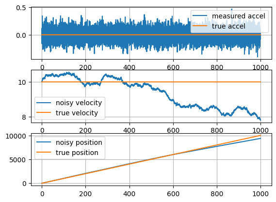
Inertial Navigation
- Inertial Measurement Unit (IMU)
- measures accelerations \(\vec{f}\)
- measures rotation rates \(\dot{\vec{\theta}}\)
- To get position from accleration, you have to integrate twice
- continuously adds noise to your position estimate
- Drifting position estimate needs to be corrected
Required data sources
- Inertial Navigation System (INS)
- Angle rates, \(\Delta\theta\)
- Accelerations/specific forces, \(\Delta\vec{v}\)
- Barometer
- Precise but not accurate
- Stablize the altitude
- Magnetometers
- Scalar - primary sensor
- Vector - for compensation
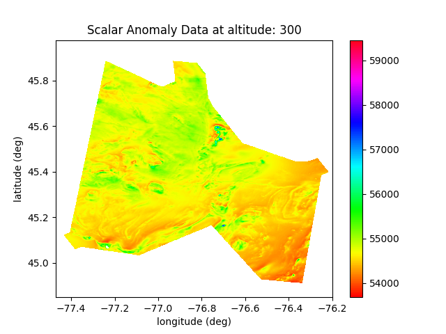
- Magnetic Map
- Core field model e.g. WMM or IGRF
- Magnetic anomaly map
Navigator overview - Extended Kalman Filter
State vector
\[
\vec{x}=
\begin{bmatrix}
\smash[b]{\underbrace{\begin{matrix}
\delta \vec{p} &
\delta \vec{v} &
\delta \vec{\epsilon} &
\vec{b}_a &
\vec{b}_g\end{matrix}}_{\text{Pinson 15}}} &
\smash[b]{\underbrace{\begin{matrix}\delta h_a &
\delta a\end{matrix}}_{\text{Baro}}} &
S_\text{fogm} &
S_\text{bias}
\end{bmatrix}
\]
Measurement processor
\[
z = h(\vec{x}) + v
\] \[
h(\vec{x}) = |B_\mathrm{a}| + |B_\text{earth}| + {\color{gray}|B_\text{Plane}}| + S_\text{fogm} + S_\text{bias}
\]
Where
- \(|B_\mathrm{a}|\) comes from map interpolation
- \(|B_\text{earth}|\) World Magnetic Model
- \(|B_\text{Plane}|\) aircraft disturbance field - not included here with SGL calibration
- \(S_\text{fogm}\) scalar state estimates of space-weather
- \(S_\text{bias}\) offset bias between map and measurement
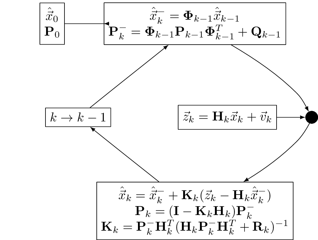
Kalman filter review
Discrete time dynamics at time index \(k+1\) the state vector \(\vec{x}_{k+1}\) is \[
\vec{x}_{k+1} = {\Phi}_k \vec{x}_k + {B}_k \vec{u}_k + \vec{w}_k
\]
- \(\Phi_k\) is the state transition matrix
- \(B_k\) is the input or control matrix
- we are not supplying control, so \(B=0\)
- \(\vec{w}\sim \mathcal{N}(0,{Q})\) is Gaussian white noise process with covariance matrix \({Q}\)
A measurement \(\vec{z}\) is \[
\vec{z}_k = {H}_k \vec{x}_k + \vec{v}_k
\]
\({H}\) is connection between state \(\vec{x}\) and measurement \(\vec{z}\)
\(\vec{v}\sim\mathcal{N}(0,{R})\) is the noise process of the measurement with covariance \({R}\)
(Brown and Hwang 2012)
The state \(\vec{x}_{k}\) has a mean \(\hat{\vec{x}}_{k}\) and covariance \({P}_{k}\) which propagates forward in time (with no other information) like: \[
\begin{aligned}
\hat{\vec{x}}_{k+1}^- & = {\Phi}_k \hat{\vec{x}}_{k} + \cancelto{0}{{B}\vec{u}_k} \\
{P}_{k+1}^- & = {\Phi}_k {P}_{k} {\Phi}_k^T + {Q}_k
\end{aligned}
\] When a measurement \(\vec{z}\) is made, we can update the propagated state vector \[
\begin{aligned}
\hat{\vec{x}}_{k} &= \hat{\vec{x}}_{k}^- + {K}_k (\vec{z}_k - {H}_k \hat{\vec{x}}_{k}^-)\\
{P}_k &= ({I} -{K}_k {H}_k ) {P}_{k}^- \\
{K}_k &= {P}_{k}^- {H}_k^T( {H}_k {P}_{k}^- {H}_k^T + {R}_k )^{-1}
\end{aligned}
\]
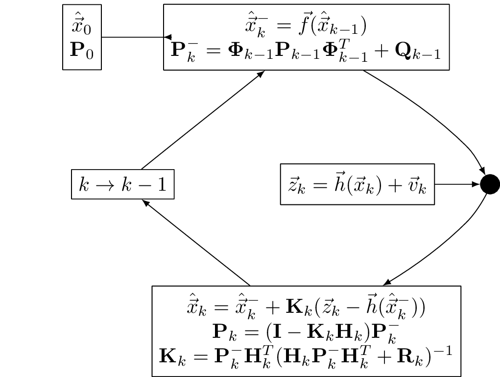
Kalman filter flow diagram
![]()
Linearization for navigation
The map-matching measurement processor is non-linear. Two primary approaches have been used for MagNav:
Generalize the state dynamics and measurement \[
\begin{aligned}
\dot{\vec{x}} & = \vec{f}(\vec{x}, \vec{u}_d, t) + \vec{u}(t) \\
\vec{z} & = \vec{h}(\vec{x}, t) + \vec{v}(t)
\end{aligned}
\]
- \(\vec{f}(\vec{x}, \vec{u}_d, t)\) and \(\vec{h}(\vec{x}, t)\) are known functions
- \(\vec{u}_d\) deterministic forcing function (e.g. gravity)
- \(\vec{u}\) and \(\vec{v}\) are uncorrelated white noise processes
Write the state \(\vec{x}\) in terms of some \(\vec{x}^*(t)\) and a deviation from it \(\Delta\vec{x}(t)\) \[
\vec{x}(t) = \vec{x}^*(t) + \Delta\vec{x}(t)
\]
Linearization of Kalman filter
\[
\begin{aligned}
\dot{\vec{x}}^* + \Delta\dot{\vec{x}} & = \vec{f}(\vec{x}^* + \Delta\vec{x}, \vec{u}_d, t) + \vec{u}(t) \\
\vec{z} & = \vec{h}(\vec{x}^* +\Delta\vec{x}, t) + \vec{v}(t)
\end{aligned}
\]
\(\Delta\vec{x}\) is small and use Taylor series (so many Taylor series) \[
\begin{aligned}
\dot{\vec{x}}^* + \Delta\dot{\vec{x}} & \approx \vec{f}(\vec{x}^*, \vec{u}_d, t) + \left[ \frac{\partial \vec{f}}{\partial \vec{x}}\right]_{\vec{x}=\vec{x}^*} \cdot \Delta\vec{x} + \vec{u}(t) \\
\vec{z} & \approx \vec{h}(\vec{x}^*, t) + \left[ \frac{\partial \vec{h}}{\partial \vec{x}}\right]_{\vec{x}=\vec{x}^*} \cdot \Delta\vec{x} + \vec{v}(t)
\end{aligned}
\] If \(\vec{x}^*\) is just a single known trajectory, then this is just the Linearized Kalman filter.
If \(\vec{x}^*\) is our trajectory estimate, then this is the Extended Kalman filter.
Equivalent linearized represenation
\[
\begin{aligned}
\dot{\vec{x}}^* + \Delta\dot{\vec{x}} & \approx \vec{f}(\vec{x}^*, \vec{u}_d, t) + \left[ \frac{\partial \vec{f}}{\partial \vec{x}}\right]_{\vec{x}=\vec{x}^*} \cdot \Delta\vec{x} + \vec{u}(t) \\
\vec{z} & \approx \vec{h}(\vec{x}^*, t) + \left[ \frac{\partial \vec{h}}{\partial \vec{x}}\right]_{\vec{x}=\vec{x}^*} \cdot \Delta\vec{x} + \vec{v}(t)
\end{aligned}
\] Becomes \[
\begin{aligned}
\dot{\vec{x}}^* + \Delta\dot{\vec{x}} & \approx \vec{f}(\vec{x}^*, \vec{u}_d, t) + \mathbf{F} \cdot \Delta\vec{x} + \vec{u}(t) \\
\vec{z} & \approx \vec{h}(\vec{x}^*, t) + \mathbf{H} \cdot \Delta\vec{x} + \vec{v}(t)
\end{aligned}
\] with \[
\mathbf{F} = \left[ \frac{\partial \vec{f}}{\partial \vec{x}}\right]_{\vec{x}=\vec{x}^*},\
\mathbf{H} = \left[ \frac{\partial \vec{h}}{\partial \vec{x}}\right]_{\vec{x}=\vec{x}^*}
\]
Extended Kalman Filter (EKF)
Write the linearized measurement as \[
\vec{z} - \vec{h}(\vec{x}^*) = \mathbf{H} \Delta \vec{x} + \vec{v}
\] The incremental estimate update at time \(t_k\) is \[
\Delta\hat{\vec{x}}_k = \Delta\hat{\vec{x}}_k^- + \mathbf{K}_k \left[ \vec{z}_k - \vec{h}(\vec{x}^*_k) - \mathbf{H}_k \Delta\hat{\vec{x}}_k^- \right]
\] Write the estimate of what the measurement should be \[
\hat{\vec{z}}^-_k = \vec{h}(\vec{x}^*_k) + \mathbf{H}_k \Delta\hat{\vec{x}}_k^-
\] And then \[
\underbrace{\vec{x}^*_k + \Delta\hat{\vec{x}}_k}_{\textstyle\hat{\vec{x}}_k} = \underbrace{\vec{x}^*_k + \Delta\hat{\vec{x}}_k^-}_{\textstyle\hat{\vec{x}}_k^-} + \mathbf{K}_k \left[ \vec{z}_k - \hat{\vec{z}}^-_k \right]
\]
EKF data flow
![]()
Pinson-9 model for inertial navigation
(Titterton and Weston 2004), (Raquet 2021)
Pinson 9-state model for INS is: \[
\vec{x} =
\begin{bmatrix}
\delta x_n \\
\delta x_e \\
\delta x_d \\
\delta v_n \\
\delta v_e \\
\delta v_d \\
\delta\epsilon_n \\
\delta\epsilon_e \\
\delta\epsilon_d \\
\end{bmatrix}
=
\begin{bmatrix}
\delta\vec{x} \\
\delta\vec{v} \\
\delta\vec{\epsilon} \\
\end{bmatrix}
\]
Where:
- \(\delta\vec{x}\) are the NED position error states
- \(\delta\vec{v}\) are the NED velocity error states
- \(\delta\vec{\epsilon}\) are the angle atittude errors
and \[
\dot{\vec{x}} = \mathbf{F} \vec{x}
\]
Imprantly \(\mathbf{F}\) is a matrix, this is not non-linear propagation.
Pinson-9 model propagation
\[
\begin{bmatrix}
\delta\dot{\vec{x}} \\
\delta\dot{\vec{v}} \\
\delta\dot{\vec{\epsilon}}
\end{bmatrix} =
\begin{bmatrix}
F_{xx} & F_{xv} & F_{x\epsilon} \\
F_{vx} & F_{vv} & F_{v\epsilon} \\
F_{\epsilon x} & F_{\epsilon v} & F_{\epsilon \epsilon} \\
\end{bmatrix}
\begin{bmatrix}
\delta \vec{x} \\
\delta \vec{v} \\
\delta \vec{\epsilon} \\
\end{bmatrix}
\] We are working in geodetic coordinates so the elements of \(\mathbf{F}\) depend upon Earth specifc parameters to account for Coriolis force.
Pinson-9 model propagation definitions
| \(\phi\) |
latitude |
radian |
| \(v_n\) |
north velocity |
meter/second |
| \(v_e\) |
east velocity |
meter/second |
| \(v_d\) |
down velocity |
meter/second |
| \(f_n\) |
north specific force |
meter/second/second |
| \(f_e\) |
east specific force |
meter/second/second |
| \(f_d\) |
down specific force |
meter/second/second |
| \(R_{\oplus}\) |
Earth radius |
635300 meter |
| \(\Omega_{\oplus}\) |
Earth rotation rate |
7.2921151467e-5/second |
Components of \(\mathbf{F}\), \(F_x\) row
\[
F_{xx} =
\begin{bmatrix}
0 & 0 & -\frac{v_n}{R_{\oplus}^2}\\
\frac{v_e \tan \phi}{R_{\oplus}\cos \phi} & 0 & \frac{v_e}{R_{\oplus}^2 \cos\phi} \\
0 & 0 & 0 \\
\end{bmatrix}
\]
\[
F_{xv} =
\begin{bmatrix}
\frac{1}{R_{\oplus}} & 0 & 0\\
0 & \frac{1}{R_{\oplus}\cos\phi} & 0 \\
0 & 0 & -1 \\
\end{bmatrix}
\]
\[
F_{x\epsilon} = \mathbf{0}_{3\times 3}
\]
\(F_v\) row of \(\mathbf{F}\)
\[
F_{vx} =
\begin{bmatrix}
v_e \left( 2\Omega_{\oplus}\cos\phi + \frac{v_e}{R_{\oplus}\cos^2\phi} \right) & 0 & \frac{v_e^2\tan\phi - v_n v_d}{R_{\oplus}^2}\\
2\Omega_{\oplus}\left(v_n \cos\phi - v_d \sin\phi\right) + \frac{v_n v_e}{R_{\oplus}\cos^2\phi} & 0 & \frac{-v_e (v_n\tan\phi +v_d)}{R_{\oplus}^2}\\
2\Omega_{\oplus}v_e \sin \phi & 0 & \frac{v_n^2 + v_e^2}{R_{\oplus}} \\
\end{bmatrix}
\]
\[
F_{vv} =
\begin{bmatrix}
\frac{v_d}{R_{\oplus}} & -2 \left( \Omega_{\oplus}\sin\phi + \frac{v_e\tan\phi}{R_{\oplus}} \right) & \frac{v_n}{R_{\oplus}} \\
2\Omega_{\oplus}\sin\phi + \frac{v_e\tan\phi}{R_{\oplus}} & \frac{v_n\tan\phi+v_d}{R_{\oplus}} & 2\Omega_{\oplus}\cos\phi + \frac{v_e}{R_{\oplus}} \\
-\frac{2v_n}{R_{\oplus}} & -2 \left( \Omega_{\oplus}\cos\phi + \frac{v_e}{R_{\oplus}} \right) & 0 \\
\end{bmatrix}
\]
\[
F_{v\epsilon} =
\begin{bmatrix}
0 & -f_d & f_e \\
f_d & 0 & -f_n \\
-f_e & f_n & 0
\end{bmatrix}
\]
\(F_\epsilon\) row of \(\mathbf{F}\)
\[
F_{\epsilon x} =
\begin{bmatrix}
-\Omega_{\oplus}\sin\phi & 0 & -\frac{v_e}{R_{\oplus}} \\
0 & 0 & \frac{v_n}{R_{\oplus}^2} \\
-\Omega_{\oplus}\cos\phi - \frac{v_e}{R_{\oplus}\cos^2\phi} & 0 & \frac{v_e\tan\phi}{R_{\oplus}^2}
\end{bmatrix}
\]
\[
F_{\epsilon v } =
\begin{bmatrix}
0 & 1/R_{\oplus}& 0 \\
-1/R_{\oplus}& 0 & 0 \\
0 & \frac{\tan\phi}{R_{\oplus}} & 0 \\
\end{bmatrix}
\]
\[
F_{\epsilon\epsilon} =
\begin{bmatrix}
0 & -\Omega_{\oplus}\sin\phi + \frac{v_e}{R_{\oplus}\tan\phi} & v_n/R_{\oplus}\\
\Omega_{\oplus}\sin\phi + \frac{v_e\tan\phi}{R_{\oplus}} & 0 & \Omega_{\oplus}\cos\phi + v_e/R_{\oplus}\\
-v_n/R_{\oplus}& -\Omega\cos\phi -v_e/R_{\oplus}& 0 \\
\end{bmatrix}
\]
Pinson-15 state model
- Extends the 9-state model to include
- accelerometer \(\vec{b_a}\) and gyro \(\vec{b_g}\) biases
- using First Order Gauss Markov model (FOGM)
\[
\vec{x} =
\begin{bmatrix}
\delta x_n \\
\delta x_e \\
\delta x_d \\
\delta v_n \\
\delta v_e \\
\delta v_d \\
\delta\epsilon_n \\
\delta\epsilon_e \\
\delta\epsilon_d \\
b_{a_x} \\
b_{a_y} \\
b_{a_z} \\
b_{g_x} \\
b_{g_y} \\
b_{g_z} \\
\end{bmatrix}
=
\begin{bmatrix}
\delta\vec{x} \\
\delta\vec{v} \\
\delta\vec{\epsilon} \\
\vec{b_a}\\
\vec{b_g}\\
\end{bmatrix}
\]
Propagation for 15-state Pinson model
\[
\begin{bmatrix}
\delta\dot{\vec{x}} \\
\delta\dot{\vec{v}} \\
\delta\dot{\vec{\epsilon}} \\
\dot{\vec{b_a}}\\
\dot{\vec{b_g}}\\
\end{bmatrix} =
\begin{bmatrix}
F_{xx} & F_{xv} & 0 & 0 & 0\\
F_{vx} & F_{vv} & F_{v\epsilon} & \mathbf{C}_b^n & 0 \\
F_{\epsilon x} & F_{\epsilon v} & F_{\epsilon \epsilon} & 0 & -\mathbf{C}_b^n \\
0 & 0 & 0 & F_{aa} & 0 \\
0 & 0 & 0 & 0 & F_{gg} \\
\end{bmatrix}
\begin{bmatrix}
\delta \vec{x} \\
\delta \vec{v} \\
\delta \vec{\epsilon} \\
\vec{b}_a\\
\vec{b}_g\\
\end{bmatrix}
\]
\[
F_{aa} =
\begin{bmatrix}
-1/\tau_a & 0 & 0 \\
0 & -1/\tau_a & 0 \\
0 & 0 & -1/\tau_a\\
\end{bmatrix},\
F_{gg} =
\begin{bmatrix}
-1/\tau_g & 0 & 0 \\
0 & -1/\tau_g & 0 \\
0 & 0 & -1/\tau_g\\
\end{bmatrix}
\] and \(\mathbf{C}_b^n\) is the direction cosine matrix that rotates from body to NED frame.
MagNav additions to Pinson-15
- Add a barometer altimeter to constrain altitude
- \(\delta h_a\) is the altitude error correction to the INS
- \(\delta a\) is the vertical acceleration error (we already have \(\delta v_n\) in Pinson-9)
- Add a state \(S\) to model external time-correlated magnetic field variations
- disturbance field e.g. diurnal variations
- effects must be out-side of navigation frequency band
Results in an 18-component state vector \[
\begin{bmatrix}
\delta \vec{x} &
\delta \vec{v} &
\delta \vec{\epsilon} &
\vec{b}_a &
\vec{b}_g &
\delta h_a &
\delta a &
S
\end{bmatrix}
\]
Updates to \(\mathbf{F}\) matrix
\[
\begin{bmatrix}
\delta\dot{\vec{x}} \\
\delta\dot{\vec{v}} \\
\delta\dot{\vec{\epsilon}} \\
\dot{\vec{b}}_a\\
\dot{\vec{b}}_g\\
\dot{h_a}\\
\dot{\delta_a}\\
\dot{S}
\end{bmatrix} =
\begin{bmatrix}
F_{xx} & F_{xv} & 0 & 0 & 0 & F_{xb} & 0 \\
F_{vx} & F_{vv} & F_{v\epsilon} & \mathbf{C}_b^n & 0 & F_{vb} & 0 \\
F_{\epsilon x} & F_{\epsilon v} & F_{\epsilon \epsilon} & 0 & -\mathbf{C}_b^n & 0 & 0 \\
0 & 0 & 0 & F_{aa} & 0 & 0 & 0\\
0 & 0 & 0 & 0 & F_{gg} &0 & 0 \\
F_{bp} & 0 & 0 & 0 & 0 & F_{bb} & 0 \\
0 & 0 & 0 & 0 & 0 & 0 & F_{ss} \\
\end{bmatrix}
\begin{bmatrix}
\delta \vec{x} \\
\delta \vec{v} \\
\delta \vec{\epsilon} \\
\vec{b}_a\\
\vec{b}_g\\
\delta h_a \\
\delta a \\
S
\end{bmatrix}
\]
Updated \(\mathbf{F}\) components
Barometer aiding: \[
\mathbf{F}_{xb} =
\begin{bmatrix}
0 & 0 \\
0 & 0 \\
k_1 & 0
\end{bmatrix},\
\mathbf{F}_{vb} =
\begin{bmatrix}
0 & 0 \\
0 & 0 \\
-k_2 & 1 \\
\end{bmatrix}
\]
\[
\mathbf{F}_{bx} =
\begin{bmatrix}
0 & 0 & 0\\
0 & 0 & k_3 \\
\end{bmatrix},\
\mathbf{F}_{bb} =
\begin{bmatrix}
-\frac{1}{\tau_b} & 0 \\
-k_3 & 0 \\
\end{bmatrix}
\]
The disturbance field bias is given by: \[
\mathbf{F}_{ss} = \frac{1}{\tau_s}
\]
MagNav measurement processor
The scalar sensor measures: \[
|\vec{B}_\text{total}| = |\vec{B}_\text{ext}+ \vec{B}_\text{\class{fa fa-plane}{}} |
\] and \[
\vec{B}_\text{ext}= \vec{B}_{\oplus}+ \vec{B}_\text{anomaly} + \vec{B}_\text{disturbance}
\]
- We added a state \(S\) into the MagNav model to account for \(\vec{B}_\text{disturbance}\).
- \(\vec{B}_{\oplus}\) from IGRF or WMM
- Both IGRF and WMM are functions of lat, long, altitude and time
- WMM has \(28.8^\circ\) or 3200 km at surface resolution
- Secular variaton \(\approx 100 \text{nT}/\text{year} = 0.27 \text{nT}/\text{day}\)
MagNav Measurement Processor \(H\) matrix
\[
\begin{aligned}
\vec{z} & \approx \vec{h}(\vec{x}^*, t) + \mathbf{H} \cdot \Delta\vec{x} + \vec{v}(t)
\end{aligned}
\]
\[
\mathbf{H} = \left[ \frac{\partial \vec{h}}{\partial \vec{x}}\right]_{\vec{x}=\vec{x}^*}
\]
\[
\mathbf{H}(\vec{x}^*) =
\begin{bmatrix}
\frac{\partial h(\vec{x}^*)}{\partial x_n} \\
\frac{\partial h(\vec{x}^*)}{\partial x_e} \\
\frac{\partial h(\vec{x}^*)}{\partial x_d} \\
\mathbf{0}_{1x15}
\end{bmatrix}
\leftarrow\text{This is the gradient of the map}
\] Both the map and 3D gradient of the map are needed in order to make a measurement and incorporate it.
Simplified sequential processing
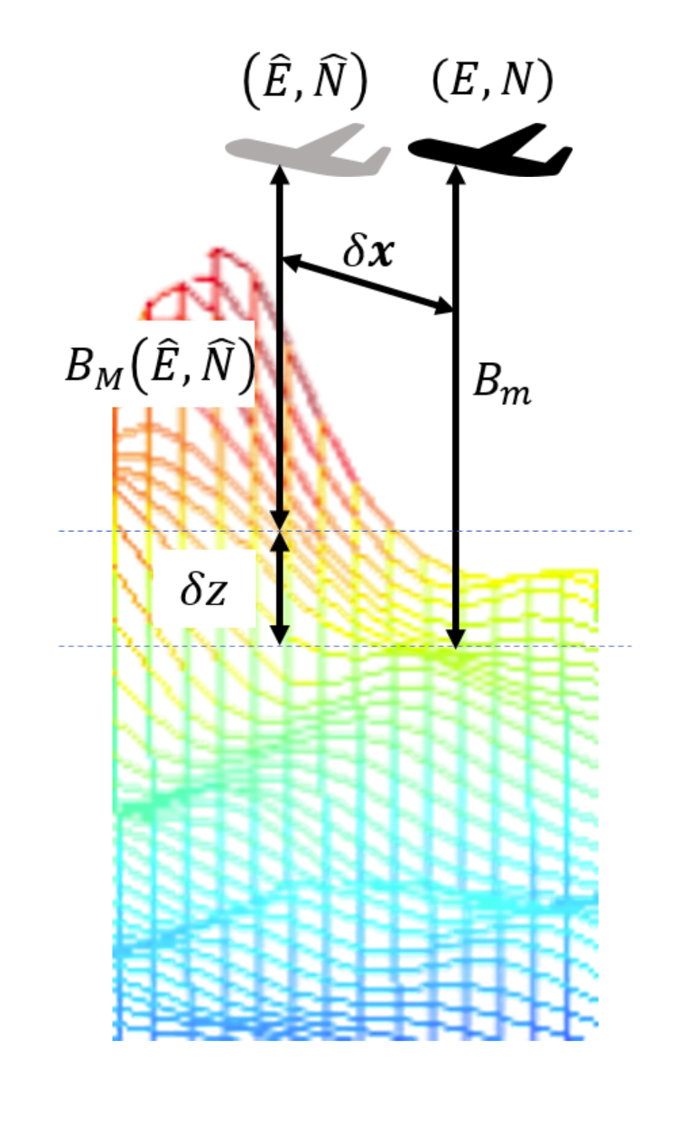
- Measurement processor: \(\delta z = B_\text{measured} - B_\text{map}(\hat{E},\hat{N})\)
- \(B_\text{measured}\) is measured magnetic field
- \(B_\text{map}(\hat{E},\hat{N})\) is the predicted map value based on position estimate
- State vector error: \(\delta \vec{x} = \left[ \delta E, \delta N \right]^T\)
- Measurement matrix: \(\mathbf{H} = \left[ \frac{\partial B_\text{map}(\hat{E},\hat{N})}{\partial E} \frac{\partial B_\text{map}(\hat{E},\hat{N})}{\partial N} \right]\)
- Measurement equation: \(\mathbf{H} \delta \vec{x}\)
- Update of the state vector error depends on the map gradients in East and North directions
Navigation pre-processor
- Prepare Magnetic Anomaly Map
- Upward continue as needed for flight altitudes
- Compute 3-D gradient for measurement processor
- Precompute Core field model as needed
- Prepare Tolles-Lawson Compensation coefficients
- In an adaptive or online calibration this is a starting point
Filter initialization
- Assume known starting value for position and attitude from GPS-aided system
- Tolles-Lawson coefficients are needed
- Works well for EKF - provides excellent starting point for state
- State starting point initializes map error state \(S\)
Cramer-Rao Lower Bound
- Cramer-Rao Lower Bound (CRLB) is the minimum theorical lowest covariance estimate
- \(\mathbf{P}_t = E\left[ ({\vec{x}_t}-\hat{\vec{x}}^-_t)({\vec{x}_t}-\hat{\vec{x}}^-_t)^T \right]\)
- Terrain-Aided Navigation (Bergman 1997)
- Magnetic Maps (Canciani 2021)
\[
\mathbf{P}_{k+1}= \mathbf{P}_k -
\mathbf{P}_k\mathbf{H}_k\left(\mathbf{H}_k^T\mathbf{P}_k\mathbf{H}_k +\mathbf{R}_k\right)^{-1}
\mathbf{H}_k^T\mathbf{P}_k + \mathbf{Q}_k
\]
\[
\mathbf{H} = \frac{\delta h^T(\vec{k})}{\delta \vec{x}_k}
\]
\[
z_t = |\vec{B}_\text{map}+ \vec{B}_{\oplus}+ \vec{B}_\text{disturbance}| + w
\]
- \(\vec{B}_{\oplus}\) varies slowly.
- Dominant term is map gradient \(\rightarrow\) limiting factor.
- Map gradient changes with altitude
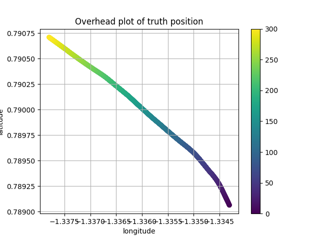
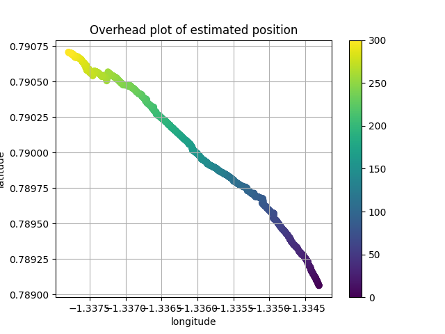
State vector comparisons
- EKF tracks Whole State (latitude/longitude) + Error state
- Taylor series expansion of the state
- Minor change is needed from Pinson model in NED to LLH
- Usually NED meters easier to interpret than LLH in radians
- Comparison to truth is also good
- Following examples come from ANT Center’s navigator running on MIT-AIA challenge problem data data
Magnetic measurement error
- Compare post-compensated magnetic signal with map value
- Differences might be due to
- poor compensation
- disturbance field changes (e.g. diurnal effects)
- map errors
- and more!
Sensor measurement to map comparison
- Need to explain at least 100 nT of error.