Sensors
ION MagNav Workshop 2023, Monterey, CA
The views expressed in this article are those of the author and do not necessarily reflect the official policy or position of the United States Government, Department of Defense, United States Air Force or Air University.
Distribution A: Authorized for public release. Distribution is unlimited. Case No. 2023-0427.
Magnetometer history
- Compass use documented in China 4th Century BCE (Yan 475-221 BCE)
- Gauss invented magnetometer in 1833 (Gauss 1833)
- Aschenbrenner and Goubau invented flux-gate magnetometer in 1936 (Aschenbrenner 1936)
- Vector sensor, measures one component of \(\vec{B}\)
- 3 sensors required to measure all components
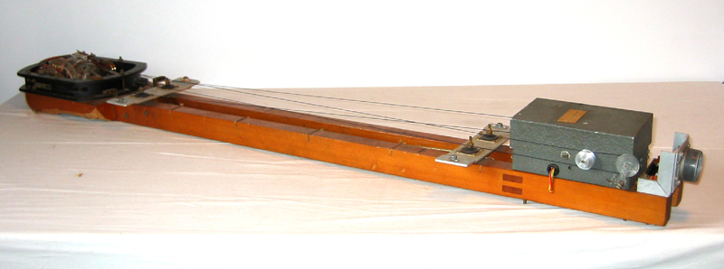
- Vacquier invented airborne version of fluxgate (Vacquier 1945)
- Used gimbal to align sensor axis with total field
- Alkali vapor magnetometers (Bloom 1962) (Bell and Bloom 1957)
- Measure vector magnitude or total field \(|\vec{B}|\)
- Review article in (Tierney et al. 2019)
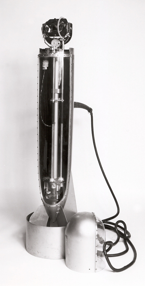
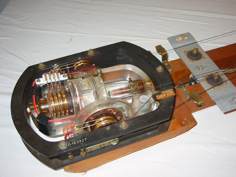
Vaquier towed magnetometer, National Museum of American History (Smithsonian Institution, n.d.)
History notes:
https://www.sciencenews.org/article/fluxgate-magnetometer-submarine-plate-tectonics
https://science.nasa.gov/technology/technology-highlights/rediscovering-the-lost-art-of-fluxgate-magnetometer-cores
https://geomag.nrcan.gc.ca/lab/vm/fluxgate-en.php
https://geomag.nrcan.gc.ca/lab/vm/museum-en.php
https://www.sciencenews.org/article/fluxgate-magnetometer-submarine-plate-tectonics
https://americanhistory.si.edu/collections/search/object/nmah_871581
https://faculty.epss.ucla.edu/~ctrussell/ESS265/History.html
https://wiki.seg.org/wiki/Victor_Vacquier
Scalar measurements
- Used traditionally to avoid need to measure true attitude in Earth frame
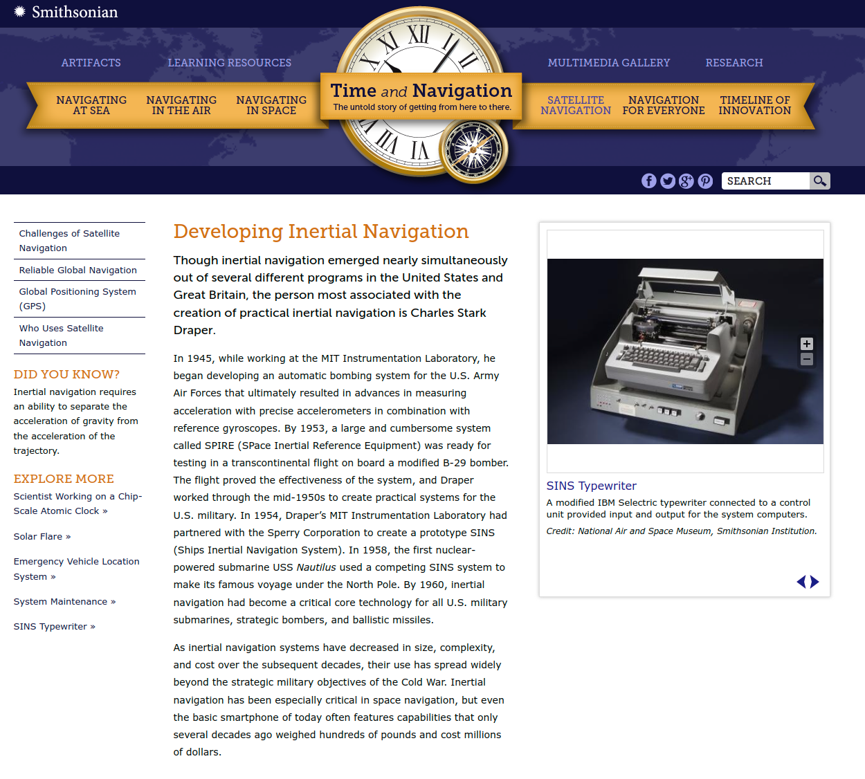
- INS not available as practical technology until 1960’s or later Smithsonian history of inertial navigation, Smithsonian Institution (n.d.)
Sensors for scalar measurements
Scalar sensors used to avoid rotation issues
Vector sensors as attitude sensors
- Could not measure your true orientation in Earth reference frame (no IMU)
- Could measure orientation around Earth field using vector sensor
- Vector could be strap-down
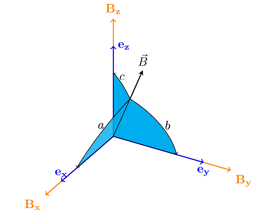
- Direction cosines used
- Tolles-Lawson calibration (W. E. Tolles and Lawson 1950) (W. E. Tolles 1954) (W. E. Tolles 1955) (Leliak 1961)
\[ \begin{align*} DC_x = \arccos{a} &= \frac{B_x}{\sqrt{B_x^2 + B_y^2 + B_z^2}}\\ DC_y = \arccos{b} &= \frac{B_y}{\sqrt{B_x^2 + B_y^2 + B_z^2}}\\ DC_z = \arccos{c} &= \frac{B_z}{\sqrt{B_x^2 + B_y^2 + B_z^2}} \end{align*} \]
Vector calibration example
- Before calibration, the vector magnetometer lies on a shifted ellipse.
- After calibration, the vector magnetomter values will lie on the surface of a sphere.
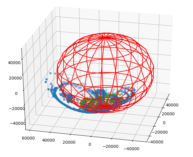
- blue - before calibration
- green -after calibration
- red - fixed magnitude sphere
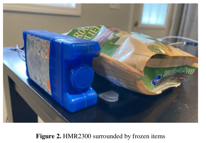
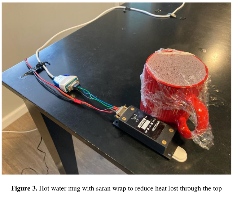
Temperature dependence
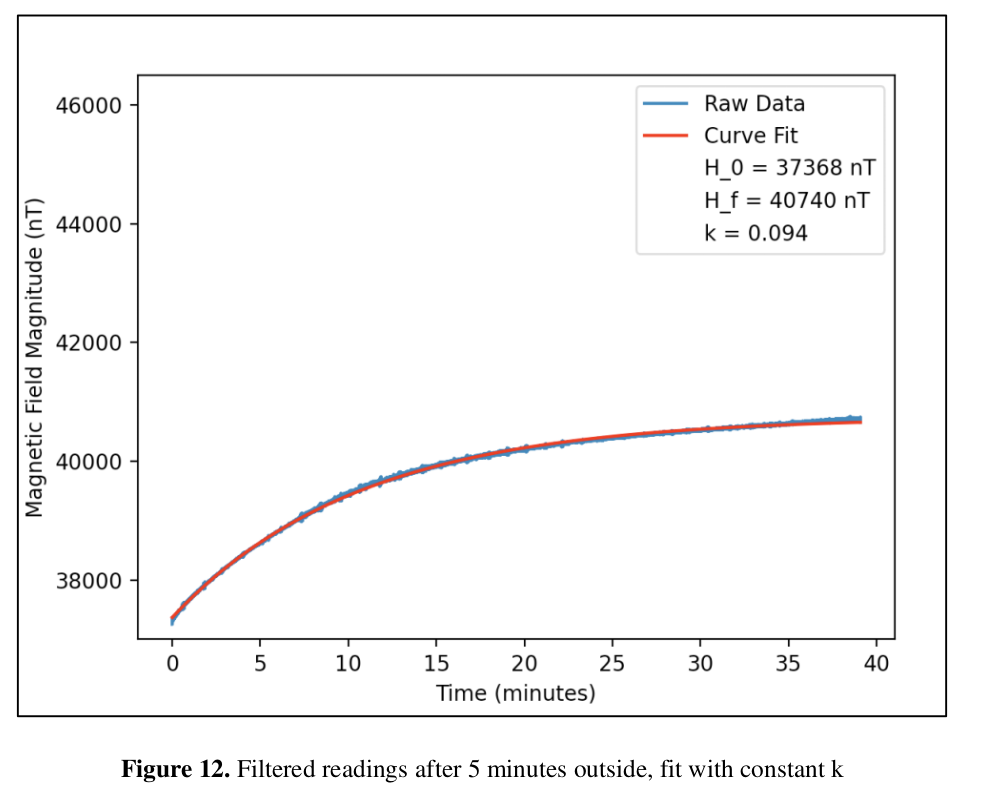
Newton’s law of cooling \[T(t) = T_s +(T_0 - T_s)\exp(-kt)\] which is the solution to \[\frac{dT}{dt} = -k(T_0 - T_s)\] if \(H \propto T\) then we can write by analogy \[H(t) = H_f + (H_0 - H_f)\exp(-kt)\]
Temperature compensation
Newton’s law of cooling \[T(t) = T_s +(T_0 - T_s)\exp(-kt)\] which is the solution to \[\frac{dT}{dt} = -k(T_0 - T_s)\] if \(H \propto T\) then we can write by analogy \[H(t) = H_f + (H_0 - H_f)\exp(-kt)\]
Scalar sensors
Scalar sensor has advantage that it’s output independent of magnetic field orientation.
Generally we refer to Atomic vapor sensors.
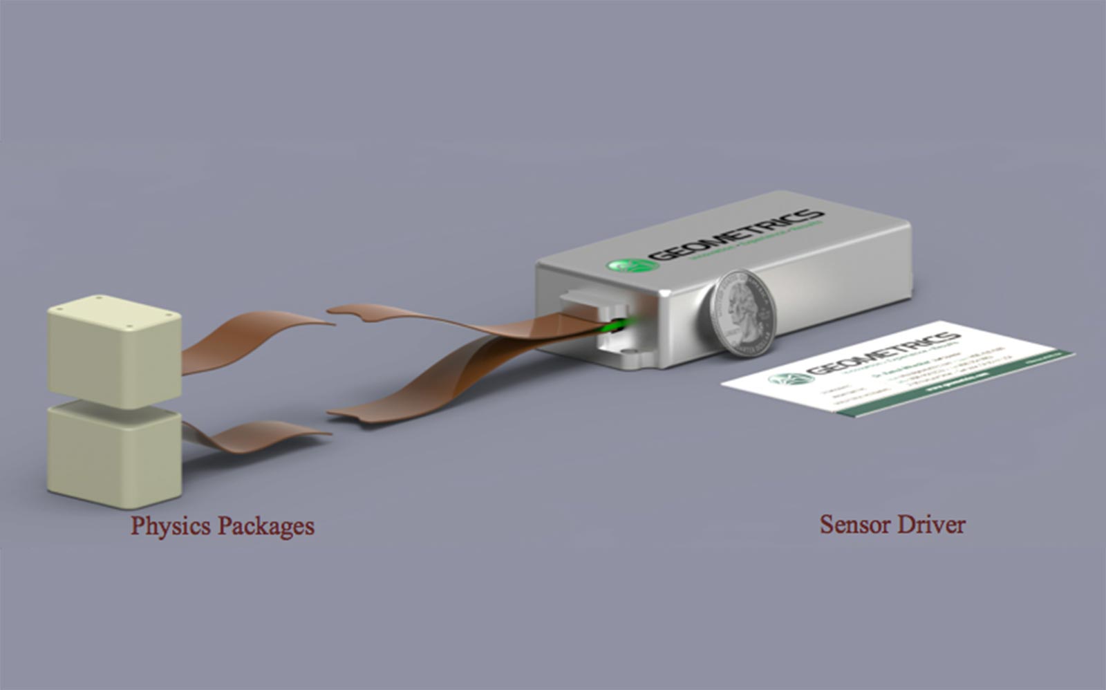
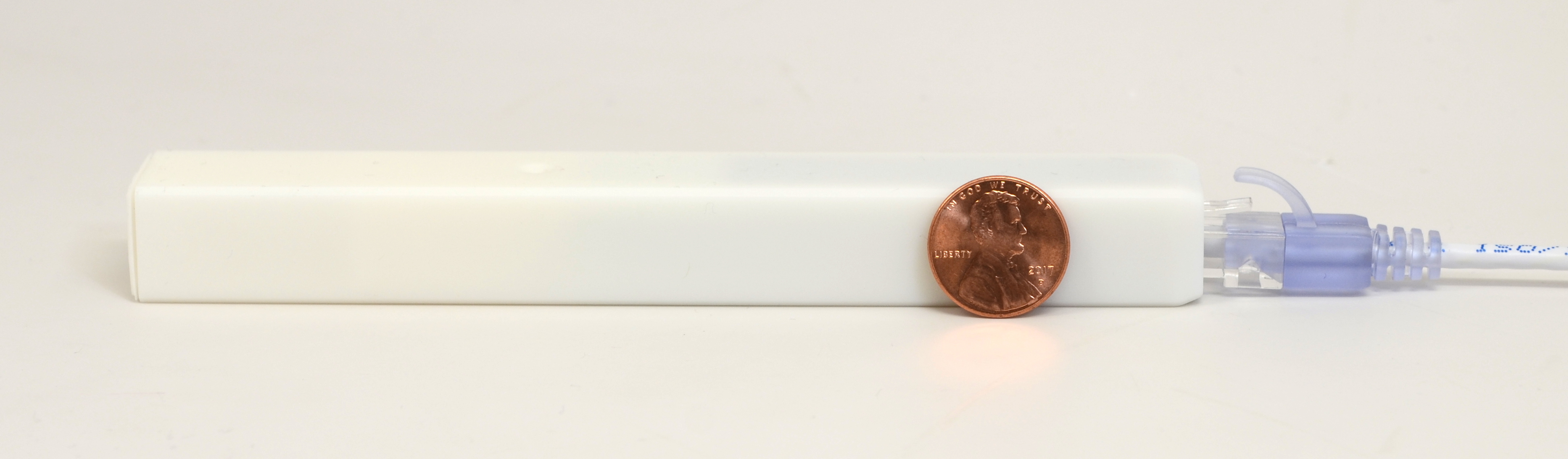
Geometrics MFAM (MFAM Module Specifications, Laser Pumped Cesium Magnetometer 2020)
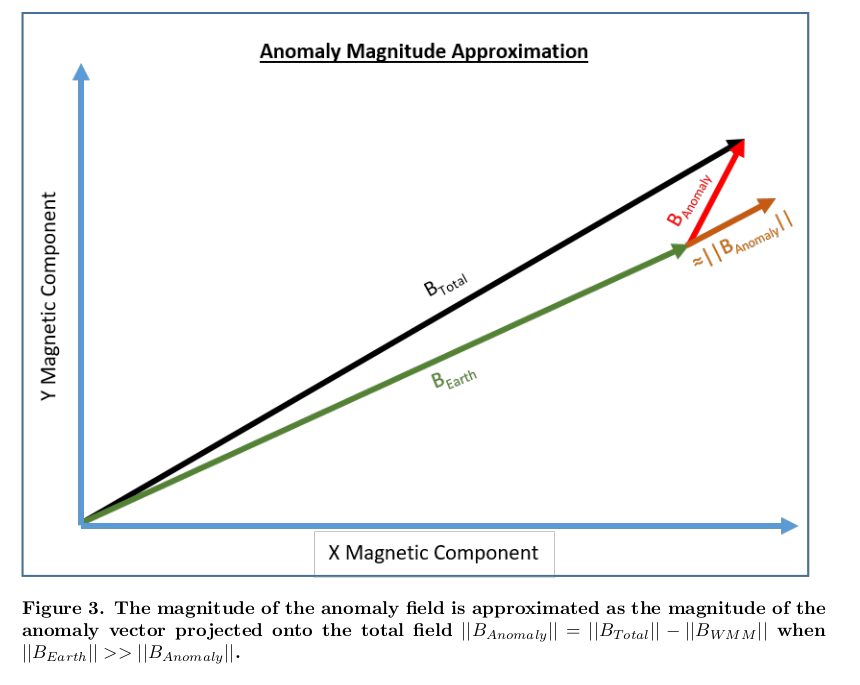
Interpretation of scalar value in geomagnetic context
\[ \begin{align*} |\vec{B}_\mathrm{total}| &= |\vec{B}_\mathrm{Earth} + \vec{B}_\mathrm{anomaly}|\\ &= \sqrt{ |B_\mathrm{Earth}|^2 + |B_\mathrm{anomaly}|^2 + 2 |B_\mathrm{Earth}||B_\mathrm{anomaly}|\cos\theta}\\ |B_\mathrm{total}| &= |B_\mathrm{Earth}| \sqrt{ 1 + \frac{|B_\mathrm{anomaly}|^2}{|B_\mathrm{Earth}|^2} + 2\frac{|B_\mathrm{anomaly}|}{|B_\mathrm{Earth}|}\cos\theta } \\ &\approx |B_\mathrm{Earth}| + |B_\mathrm{anomaly}|\cos\theta + \cdots \end{align*} \]
\(|B_\mathrm{anomaly}|\) is the projection of \(\vec{B}_\mathrm{anomaly}\) onto \(\vec{B}_\mathrm{Earth}\)
Atomic sensors - Larmor precession
Atomic vapor sensors operate on the principle of Larmor precession
These are gases that have an unpaired electron that has a specific magnetic moment.
Cesium \(\gamma = 3.5\ \text{nT/Hz}\)
In Earth field of \(50000\ \text{nT} \rightarrow 175 \text{kHz}\)
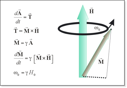
- \(\vec{A}\) is angular momentum
- \(\vec{T}\) is torque
- \(\vec{M}\) is magnetic moment
- \(\vec{H}\) is magnetic field
- \(\gamma\) is gyromagnetic ratio
Atomic sensor operation
Inside the sensor head is the Ce gas. Without doing anything the atoms in the gas have a random orientation.
A pump laser with a specific polarization orients the Ce spins and excites them to a specific state.
A probe laser reads out the precesion rate and the magnetic field is inferred.
The probe laser is polarized so that it is absorbed by the Ce gas when the spin aligns with the beam polarization.
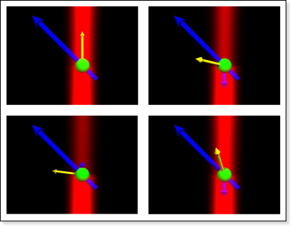
- Geometrics
- Red - probe laser beam
- Blue - magnetic field
- Yellow - magnetic moment
Deadzone
Related to the pump laser optical axis.
Pump laser is circular polarized and transfers angular momentum to the atoms so that they spin align to the optical axis \((\vec{M}\parallel\text{optical\ axis})\)
Torque \(\vec{T}\) on \(\vec{M}\) from \(\vec{H}\) is: \[ \vec{T} = \vec{M} \times \vec{H} \] If \(\vec{M} \parallel \vec{H}\), then \(\vec{T} = \vec{M} \times \vec{H} = 0\)
No torque \(\rightarrow\) no precession and no signal to monitor.
Details of laser-gas interaction define deadzone size.
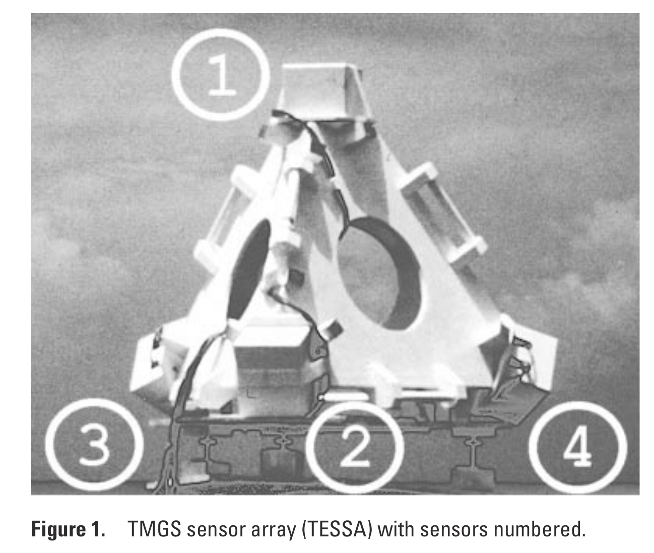
Deadzone avoidance
- Orient optical axis based on knowledge of external field
- OK if external field does not move - not practical for vehicles
- Use multiple sensors
- arrange so that one is always out of deadzone, how many do you need?
- travel from Northern to Southern hemisphere
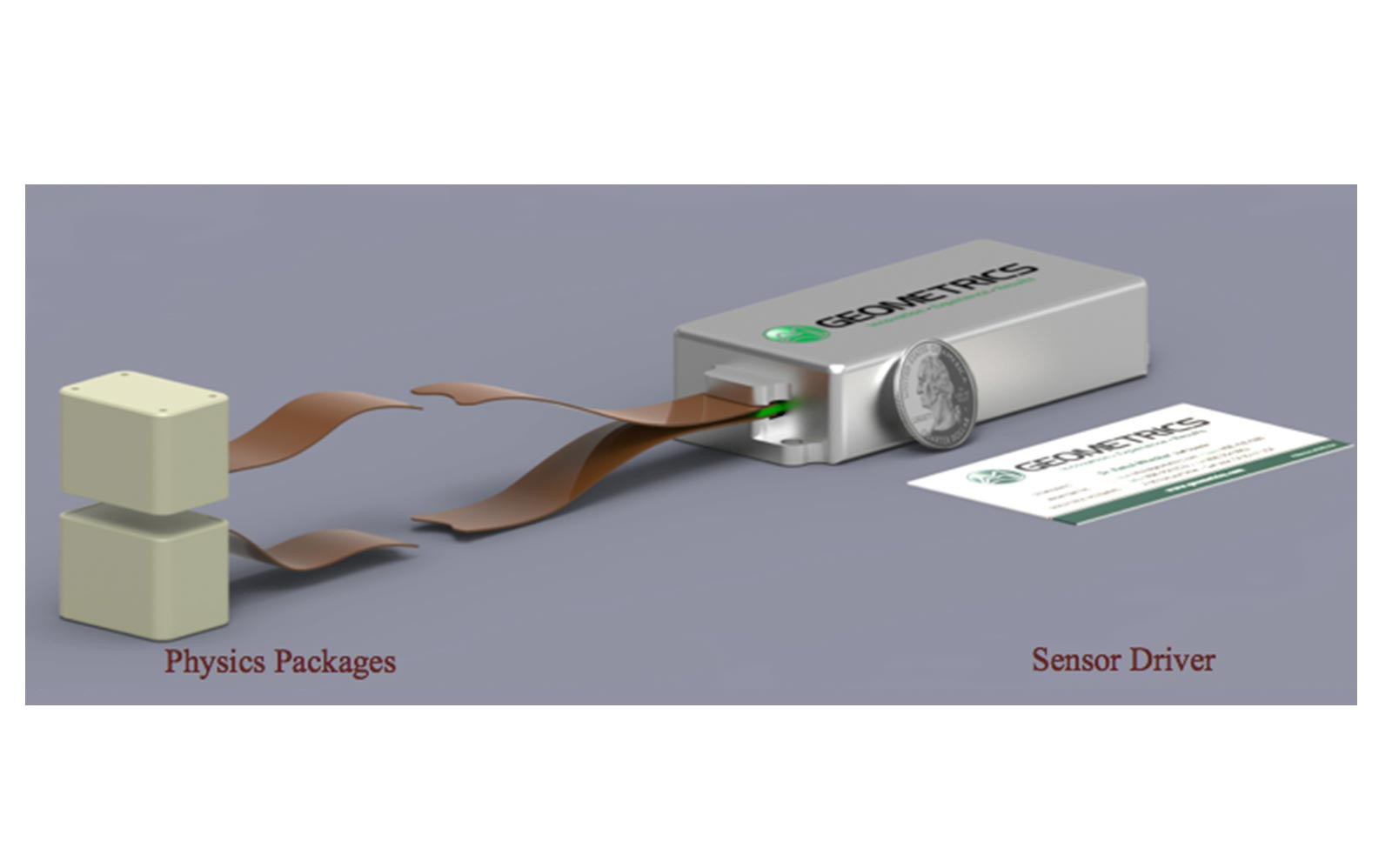
Geometrics MFAM (MFAM Module Specifications, Laser Pumped Cesium Magnetometer 2020)
Vector Gradiometer aka Tensiometer
Because of the contraints, a vector gradiometer can be made with \(\ge 4\) vector sensors in a cross (plane) or in a tetrahedron or similar shape.
 From
From 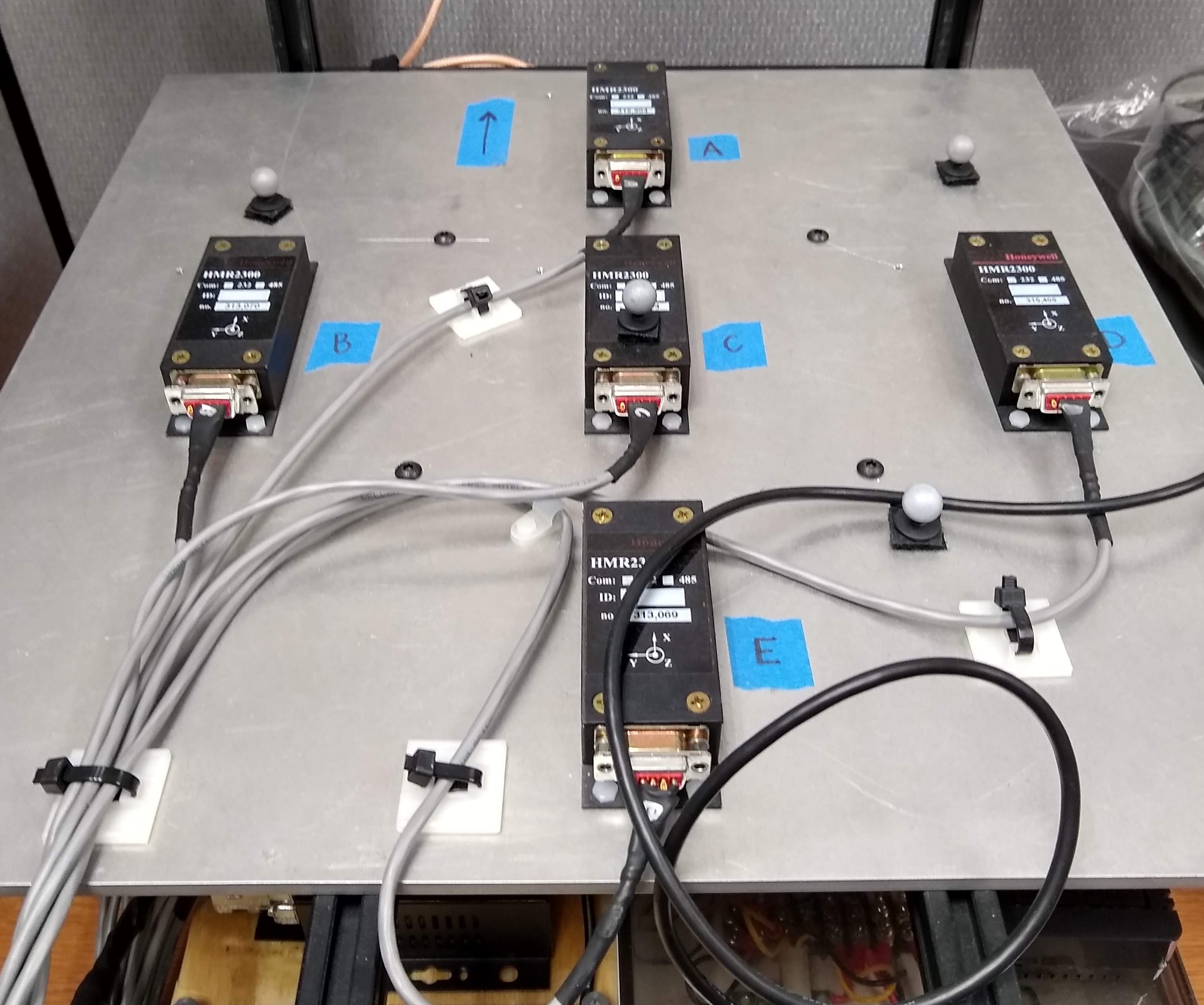
References